Across methods of matrix decomposition (ICA, Archetypal Analysis, NNMF), we run into the problem of needing to know how many signals to decompose our data to. This is called model order selection. If we choose a number that is too small (underestimation) then we lose information and our decomposition is sub-optimal. If we choose a number that is too big (overestimation), we create a bunch of spurious components and overfit the data. As a reminder, these methods assume that our data (X) is some linear combination of some N “true” signals (S), meaning that:
X = WS
where W is a matrix of weights that we apply to our matrix of signals to mix things up a bit. In the case of ICA we assume that these signals are independent, and for the other two methods we do not assume independence, but we start with positive data so our matrix of weights is also positive.
How do we do ICA in the presence of Gaussian noise?
Since ICA is either maximizing the independence of the signals by way of kurtosis maximization / minimization, entropy maximization (Infomax algorithm), or neg-entropy maximization (FastICA), shouldn’t it make sense that if we have noise (which has a Gaussian distribution), this messes up the method? Well, we could allow for one signal with a Gaussian distribution, but as we remember that any Gaussian can be expressed as the combination of other Gaussians, we can’t have more than one, otherwise we can’t unmix the signals. So, in the case of multiple Gaussians thrown into the mix, we need methods that deal with this, or methods that can accurately estimate the amount of Gaussian noise. With the standard Infomax approach applied to neuroimaging data, we don’t model the noise. We in fact assume that the data can be completely characterized by the mixing matrix and the estimated sources. What this means in fMRI is that we tend to overfit our model to noisy observations. This is when the famous Beckmann and Smith decided to create a probabilistic model that can control the distinction between what can be attributed to noise, and what can be attributed to real effects.
An ICA Method that will estimate order
This model assumes that the data is confounded by noise, and is going to help us generate our probabilistic model. This model takes three steps to estimate sources:
- We first estimate a signal and a noise subspace. Specifically, we find the signal space with probabilistic Principal Component Analysis (PPCA), and the noise subspace is orthogonal to this signal space. In this step we will estimate our number of components.
- We then estimate our sources (with FastICA)
- We then assess if the estimated sources are statistically significant
(I will discuss PICA and PPCA in detail in another post) - for now let’s start with this as our framework, and know that by using the probabilistic ICA model (PICA) we a specified order, q, we will get a unique solution.
Normalize the data
As a preprocessing step, although this may make some squirmy, we normalize the original data timecourses (meaning each voxel over time) to have zero mean and unit variance (this means subtracting the mean and dividing by the standard deviation). This assumes that all voxel’s time courses are generated from the same noise processes. We do this because, in this space, any component that isn’t noise will need to jump out and say “Hello, look at me! I’m non-Gaussian!”
Model order selection
We figure out the dimensionality of our decomposition based on the rank of the covariance matrix. Remember that covariance is a measure for how much two variables change together. If change in one variable changes the other by the equivalent amount, covariance = 1. If there is an equivalent change in the other direction, covariance is -1. If one variable doesn’t influence the other at all, covariance is 0. So if our observations are in a vector, xi, then we want to create a matrix that, in any coordinate ij, specifies the covariance between the point xi and the point xj (and remember in this case, a “point” is referring to a voxel location). If we have absolutely no noise, we know that the quantity q (the correct dimensionality) is the rank of the covariance of the observations:
Our observations, x, have length m (the number of timepoints), and this results in a mixing matrix of size mxm, so the rank is m, so our dimensionality, q, is q = m:

The equation above says that the rank of x is the rank of the dot product of the vector xi, which is the same as our mixing matrix A. However, in the presence of noise, this means that the eigenvalues of the covariance matrix are raised by adding some sigma squared:

This is really thick reading, but I will do my best to explain how I think this works. The covariance matrix, Rx, is a square matrix so it can be expressed in terms of its eigenvectors and eigenvalues. If you look at the relationship between eigenvalues/vectors and the original square matrix, multiplying the eigenvectors by the matrix of eigenvalues (down the diagonal, like a trace) is equivalent to multiplying the original matrix by the eigenvectors. I think this abstractly implies that the eigenvalues can be used as a representation of the original matrix, Rx. In this case, if we were to find identical eigenvalues, arguably, this is repeated information. And so finding the correct dimensionality, or the rank, of the matrix Rx boils down to finding the number of identical eigenvalues. However, in the case of noisy data (like fMRI) this becomes problematic because we can’t look for “exact” equality, we have to assess equality within some threshold. We need a statistical test for the equality of these values beyond some threshold.
Using prediction likelihood as a test for equality
We could decide to choose our threshold for assessing if two eigenvalues are “close enough” to be equal –> choosing the rank of the covariance matrix –> choosing the correct ICA dimension based on maximizing the likelihood of our original data, X. Would that work? It would mean going through a range of thresholds, applying them to our eigenvalue and vector matrices to reproduce the “new” (reduced) covariance matrix, and then seeing what percentage of variance our model accounts for out of the total variance of the data. I’m guessing that since the covariance matrix is simply a generalization of variance to multiple dimensions, a simple method would be to assess [total variance of thresholded model]/[total variance of original model] and try to maximize that. But wait a minute, doesn’t that mean that we could just keep decreasing the threshold (adding more eigenvalues and thus increasing the rank and proposed dimension) and we would obviously be better approximating the original data and probably get up to accounting for 99.9% of the original variance with our model? I think so. That doesn’t help us to estimate the “true” dimension of the data. What else has been proposed?
Using the “scree plot” to determine meaningful eigenvalues
A scree plot shows the ordered eigenvalues on the Y axis, and components on the X axis. It was suggested that finding a “knee” in this plot is akin would be a good way to estimate the correct dimensionlity, because some true N eigenvalues are meaningful about the data, and then when the values drop off, beyond that “knee” are junky ones. If you look at the first page of FSL’s MELODIC tool (that performs ICA with this automatic estimation, shown below), you will see this scree plot:

The eigenvalues (purple line) decrease as we move from left to right, and with this we like to see the percentage variance that our choice of dimensionality accounts for (the green line). Obviously if we include all the components (meaning that we don’t filter out any eigenvalues and the covariance matrix is assessed at its original rank) we account for 100% of the variance. But as stated previously, accounting for 100% variance in the model is not akin to finding the correct dimension of the data! In the case of the chart above, you can see why using the “knee” of the scree plot to estimate dimensionality is considered “fudging.” Is it around 4ish? 6ish? Closer to 12? Clearly this is not reliable or robust. Wait, what is that funky red line, the “dim. estimate” referring to? Maybe a better way to estimate the dimensionality!
Random matrix theory to estimate dimensionality?
Before I discuss the approach that FSL’s software uses, I want to review how random matrix theory can help us. Actually, I don’t claim to have a solid definition for what random matrix theory is, but it looks like it means filling up a matrix with random numbers from some specified distribution. In this case, it looks like if we had completely Gaussian noise, our covariance matrix would follow a particular distribution called a Wishart Distribution. We can then look at the eigenvalues for this “base case” covariance matrix that is all noise, and compare to our covariance matrix, which has some true signal + noise. The eigenvalues that are in our model but not encompassed in the eigenspectrum of an equivalently sized random Gaussian matrix, then, are the meaningful ones reflective of of the true signal.
Order Selection in a Bayesian Framework
This is the method that FSL actually uses (I believe), and it was proposed by Minka in 2000 in this paper. Minka presented a Laplace approximation to the posterior distribution of the model evidence (e.g., how many eigenvalues to include). Again, we are going to work with the eigenspectrum of the covariance matrix (Rx) to figur this out. Let’s walk through this. Since this is a bayesian approach, we want to maximize the probability of our data, X, given our choice of dimensionality, q:
| P(X | q) |
This means that we will need to define some uniform prior over all possible eigenvector matrices.
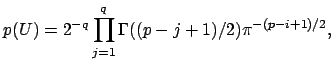
I’m not going to pretend to be able to explain this equation, I need a few hours to walk through the paper that I linked above. Intuitively, we can see that we are summing over possible square eigenvector matrices from size j=1 to the full size, q. This equation is described as “the recipricol of the manifold” as defined by James in 1954. Look at page 5 here, or the James paper here. Having only taken introductory stats courses in my life, I’m going to take the equation above as is, it is our prior to represent the summed probability of all our eigenvector matrices. We then can model the probability of our data, X, given a value of q as follows:
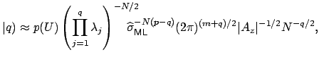
where
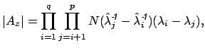
These equations look like death! For full details about the variables, see here. Basically, we find the correct dimensionality by choosing q that maximizes this equation. I’m guessing that the red line in the plot above is reflective of this changing probability, but I’m not sure.
A final note about the big picture
I’m someone that likes details, and so I am prone to get lost in said details and completely forget about the big picture. It’s a fulfilling and frustrating thing. On the one hand, it feels great to dig into something and truly understand it. On the other hand, being human means that there are only so many hours per day to distribute between work and study, and so those hours must be allocated to maximize efficiency, or doing the things that I need to do in order to be a successful researcher and student. For any topic that we learn about, you can imagine a plot of time spent on the x axis, and payoff on the y axis. When we first start to learn about some new thing, there is huge payoff, but then the payoff drops with each additional unit of time until we reach some point when it doesn’t make sense to keep learning. And so for a detail oriented person, this is a very frustrating point. It means that at some point many things turn into a black box, and unless I want to unwisely allocate my time, I have to settle and take some things at face value. Time would be much better spent learning other things that present with the same much higher initial payoff.
On the other hand, learning about algorithms is a lot like being a runner, and taking runs and bike rides to learn about a new city. The new city is a method, and the intricate corners and streets represent the depth that I understand said method. On my first outing, I choose a relatively safe route that sticks to main roads, and gives me the general gist of a city. Along the way I see many interesting places off to the side that, perhaps at some later date, I can come back to explore. On subsequent runs I go back to these places and learn more about the city. However, no matter how many times that I can go out, I have to accept that it is not feasible to inspect every atom of every corner of every building. Black box.
Suggested Citation:
Sochat, Vanessa. "Dimensionality Estimation of ICA with Bayesian Analysis." @vsoch (blog), 04 Aug 2013, https://vsoch.github.io/2013/dimensionality-estimation-of-ica-with-bayesian-analysis/ (accessed 14 Jul 26).