I’m sure that you’ve heard of the cocktail party problem. The simplest version of the problem posits that you have two people talking in a room with two microphones, each recording a mixed signal of the two voices. The challenge is to take these mixed recordings, and use some computational magic to separate the signals into person 1 and person 2. This is a job for independent components analysis, or ICA. ICA is only related to PCA in that we start with more complex data and the algorithm finds a more simplified version. While PCA is based on finding the main “directions” of the data that maximize variance, ICA is based on figuring out a matrix of weights that, when multiplied with independent sources, results in the observed (mixed) data.
Below, I have a PDF handout that explains ICA with monkeys and looms of colorful strings. I’ll also write about it here, giving you two resources for reference!
What variables are we working with?
To set up the ICA problem, let’s say we have:
- x: some observed temporal data (let’s say, with N timepoints), each of M observations having a mix of our independent signals. x is an N by M matrix.
- s: the original independent signals we want to uncover. s is an N x M matrix.
- A: the “mixing matrix,” or a matrix of numbers that, when multiplied with our original data (s), results in the observed data (x). This means that A is an N by N matrix. Specifically,
x=As
What do the matrices look like?
To illustrate this in the context of some data, here is a visualization of the matrices relevant to functional MRI, which is a 4D dataset consisting of many 3D brain images over time. Our first matrix takes each 3D image and breaks it into a vector of voxels, or cubes that represent the smallest resolution of the data. Each 3D image is now represented as a vector of numbers, each number corresponding to a location in space. We then stack these vectors on top of one another to make the first matrix. Since the 3D images are acquired from time 0 to N, this means that our first matrix has time in rows, and space across columns.

The matrix on the far end represents the independent signals, and so each row corresponds to an independent signals, and in the context of using fMRI data, if we take an entire row and re-organize it into a 3D image, we would have a spatial map in the brain. Let’s continue!
How do we solve for A?
We want to find the matrix in the middle, the mixing matrix. We can shuffle around some terms and re-write x = As as s = A-1x, or in words, the independent signals are equal to the inverse of the mixing matrix (called the unmixing matrix) multiplied by the observed data. Now let’s walk through the ICA algorithm. We start by modeling the joint distribution (pdf) for all of our independent signals:

In the above, we are assuming that our training examples are independent of one another. Well, oh dear, we know in the case of temporal data this likely isn’t the case! With enough training examples (e.g., timepoints), we will actually still be OK, however if we choose to optimize our final function with some iteration through our training examples (e.g., stochastic gradient descent), then it would help to shuffle the order. Moving on!
Since we already talked about that x (our observed data) = As = A-1s, let’s plug this into our distribution above. We know that s = some vector of weights applied to the observed data, and let’s call our un-mixing matrix (A inverse), W.

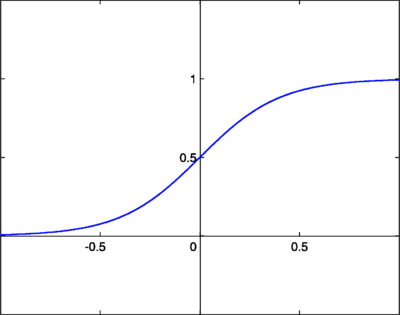
we now need to choose a cumulative distribution function (cdf) that represents the density for each independent signal. We need a CDF that increases monotonically from 0 to 1, so we choose good old sigmoid, which looks like this:
Now we should re-shift our focus to the problem above as one of maximum likelihood. We want to maximize the log likelihood parameterized by our mixing matrix W:

Remember that the cursive l represents the log likelihood. The function g represents our Sigmoid, so g prime represents the derivative of Sigmoid, which gets at the rate of change, or the area under the curve (e.g, density). By taking the log of both sides our product symbol (the capital pi) has transformed into a summation, and we have distributed the log on the right side into the summation. We are summing over n weights (the number of independent components) for each of m observations. We are trying to find the weights that maximize this equation.
Solving for W with stochastic gradient ascent
We can solve the equation above with stochastic gradient ascent, meaning that our update rule for W on each iteration (iterating through the cases, i) is:

the variable in front of the parentheses is what we will call a learning rate, or basically, how big we take a step toward our optimized value after each iteration. When this algorithm converges, we will have solved for the matrix W, which is just the inverse of A.
Finally, solve for A
When we have our matrix, A inverse (W), we can “recover” the independent signals simply by calculating:
 = Wx(i)")
Awesome!
Some caveats of ICA:
There is more detail in the PDF, however here I will briefly cover some caveats:
- There is no way to recover any original permutation of the data (e.g., order), however in the case of simply identifying different people or brain network, this largely does not matter.
- We also cannot recover the scaling of the original sources.
- The data must be non-Gaussian
- We are modeling each independent signal with sigmoid because it’s reasonable, and we don’t have a clue about the real distribution of the data. If you do have a clue, you should modify the algorithm to use this distribution.
Summary
ICA is most definitely a cool method for finding independent signals in mixed temporal data. The data might be audio files with mixtures of voices, brain images with a mixture of functional networks and noise, or financial data with common trends over time. If you would like a (save-able) rundown of ICA, as explained with monkeys and looms of colorful strings, please see the PDF below.
Suggested Citation:
Sochat, Vanessa. "Independent Component Analysis (ICA)." @vsoch (blog), 15 Jun 2013, https://vsoch.github.io/2013/independent-component-analysis-ica/ (accessed 14 Jul 26).