I was inspired by the recently shared Color Julia Bot. I didn’t realize how beautiful Julia Sets are, and I didn’t really have much understanding about how to generate them. This of course made me dive into a focused interest loop of programming for the last few days to have some fun. :)
What did I want to do?
I wanted to make a Juliart Python module that would generate basic Julia Set Images, but also:
- allow for custom coloring (themes or specific colors)
- create animations across some subset of parameters
- understand how varying parameters ca, cb changes the image
- add messages to some coordinate in the space
- understand the basics of Mandelbrot and Julia Sets
The last point resulted due to a need to figure out the other ones. I’ll go through some of these points in this post, albeit not in that exact order. For more details, see the repository.
Too Long, Didn’t Read!
If you just want to jump in, you can install juliart and then generate or animate.
pip install juliart
pip install juliart[animate]  # animation too!

juliart animate
juliart generate
There are substantial more instructions in the repository readme. For now, let’s talk about the last point.
Understanding Mandelbrot and Julia Sets
Mandelbrot Set
A Mandelbrot set is a collection of complex numbers (real numbers plus the dimension with i’s). You can imagine an axis of real numbers, and an axis of imaginary numbers perpendicular to it, and then some number of coordinates in that space below. What determines if a coordinate belongs? It means that if we start with the equation:
\begin{align} f(z) = z^2 + c \end{align}
and plug in some value of c, we can continually plug in the answer to the function again, and a member of the
Mandelbrot set will never go above 2. For example, let’s say we start with c = 1 + 0i (the 0i goes away) and z = 0
We want to know if 1 is in the set. We would first do:
\begin{align} f(z) = 0^2 + 1 \end{align}
which is equal to 0 + 1 = 1! Now we would do the same and plug in 1 for z:
\begin{align} f(1) = 1^2 + 1 \end{align}
And we get f(1) = 2. We continually plug in our answer as the new value of Z and keep going
\begin{align} f(z) = 0^2 + 1 = 1 \newline f(1) = 1^2 +1 = 2 \newline f(2) = 2^2 +1 = 5 \newline f(5) = 5^2 +1 = 26 \newline \end{align}
Remember that we are trying to determine if a particular value of c is in the Mandelbrot set.
How do we know? A number c in the Mandelbrot set, when subjected to this procedure,
will never go above 2. This means that 1 is not part of the Mandelbrot set!.
It’s going to continue to grow, unbounded. But let’s try for negative 1, meaning that c = -1 + 0i
\begin{align} f(z) = 0^2 + -1 = -1 \newline f(-1) = -1^2 + -1 = 0 \newline f(0) = 0^2 + -1 = -1 \newline f(-1) = -1^2 + -1 = 0 \newline \end{align}
Holy cow, do you see that it will keep going back and forth between 0 and -1? We can easily see that since the procedure won’t grow without bounds and definitely will never result in a value greater than two. This value of c is a member of the Mandelbrot set. If you want to see a really fantastic video about Mandelbrot sets, look no further!
Julia Sets
Now that we understand the Mandelbrot set, let’s discuss Julia Sets! The formula for the Julia set was derived by Gaston Julia. The Julia Set is a series of fractals that are generated with the same recursive formula as before, and the only difference is how we use the equation. Let’s step back. The Mandelbrot set is the set of parameters c for which the recursive relation \begin{align}z_n = f(z_{n-1}) = z_{n-1}^2 + c\end{align} does not diverge starting with \begin{align}z_0 = 0\end{align} For example, to determine if c=1 is in the set, we computed
\begin{align} z_1 = f(z_0) = z_0^1 + 1 = 1, \newline z_2 = f(z_1) = z_1^1 + 1 = 2. \newline \end{align}
Eventually we see it diverges, so it’s c = 1 is not in the Mandelbrot set.
To compute the Julia set, we instead fix the recursive relation. For example, we could choose c=1, and the Julia set to consider will correspond to the relation \begin{align}f(z) = z^2 + c\end{align} The values to be considered are not the c-values (which have now been fixed) but instead the set of starting points z0. For the Mandelbrot set, we just set this to zero, but now we vary this value instead. The plot to generate shows whether starting at any given value of z and using the recursive relation (same as before) ends up diverging or not. So for example, we already know from the previous calculation that if we start with z = 0, we get a diverging value. Before, this told us that c = 1 does not belong in the Mandelbrot set. However, from the perspective of the Julia set, this tells us about the value at the point z=0 having fixed the relation \begin{align}f(z) = z^2 + c\end{align} We can consider other initial values of z for the fixed value c = 1, which tell us about which other points are in the Julia set with our fixed relation \begin{align}f(z) = z^2 + c\end{align} but these calculations don’t say anything for the Mandelbrot set which had fixed the initial point to zero.
How do we visualize?
How do we make a pretty picture? The easiest way for me to explain in a text document is to walk through code.
# Iterating through pixels in the image (the resolution)
# See https://en.wikipedia.org/wiki/Julia_set#Pseudocode
for x in range(self.res[0]):     # real axis
    for y in range(self.res[1]): # imaginary axis

        # Scaled x and y coordinate of pixels
        za = self.translate(x, 0, self.res[0], -zoom, zoom)
        zb = self.translate(y, 0, self.res[1], -zoom, zoom)
        i = 0

        # iterations are the number of recursions of the formula we want to do
        # we consider za the real component, and zb the imaginary component
        # see https://www.youtube.com/watch?v=fAsaSkmbF5s for how equations derived
        while i < iterations:
            tmp = 2 * za * zb
            za = za * za - zb * zb + self.ca
            zb = tmp + self.cb

            # Check if the new point is outside radius R=2
            if sqrt(za * za + zb * zb) > 4:
                break
            i += 1

        # When we get here, we have a value of i (when the loop broke)
        # if i isn't the max iterations, we color it. Otherwise, it's black
        self.draw.point(
            (x, y),
            self.colorize(i, iterations) if i != iterations else (0, 0, 0),
        )
For the coloring part, if we escape the radius R=2 early (the loop breaks), we color according to how many iterations it took to escape. In the case that i == the number of iterations, this means that we got through all the iterations without escaping the radius R = 2. In this case we color black. This gave me the insight that if we want more interesting images (more opportunities to escape the radius and be given a color) we should increase the number of iterations and/or radius. One of the reasons that I really like Julia Sets is that there are so many parameters you can vary. Gosh, I haven’t even tried them all! I’m really not doing them justice with this library, but I did my best for a small project.
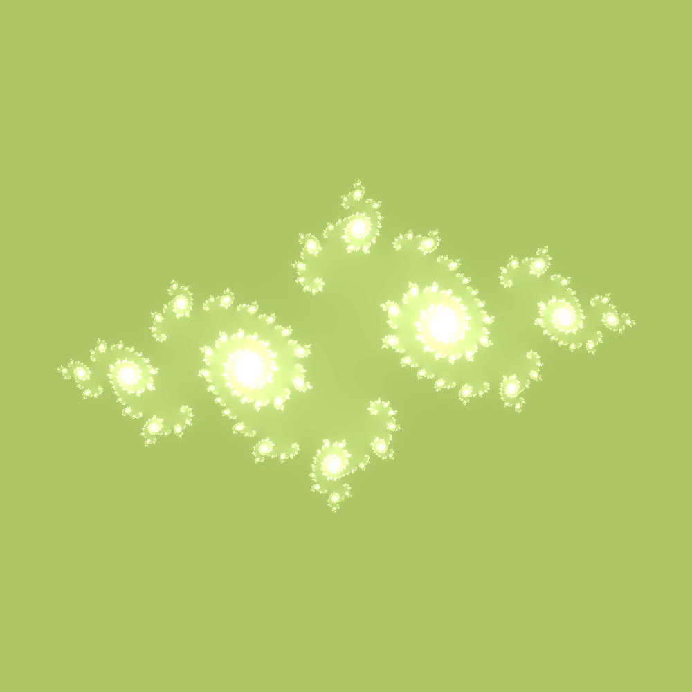
How does varying ca and cb influence the image?
I wanted to better understand how my ranged or randomly chosen choice of ca and cb (both in range (-1,1) would influence the image. I’m a more applied thinker, so I decided to just visualize it:

And here is an animation cycling through the parameter space at 1 second intervals:
And you can see the fully interactive version here. Do you see what I saw? My tiny little dinosaur brain went pouf! because I could immediately see that the Julia Sets form indices of a larger Mandelbrot set! Awesome.
Animations!
By far, the most fun kind of generation I’ve done is animations! Here is a random sampling:

You can add text to an animation or static image (here is the animation):

And you can see more examples in this folder. Some can be very flashy, and others not. The resolution (based on number of frames and randomly selected parameters) can vary a bit.

Other Examples
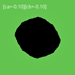
Here is an example of a pattern generation. We set a hard threshold and color black or a color.

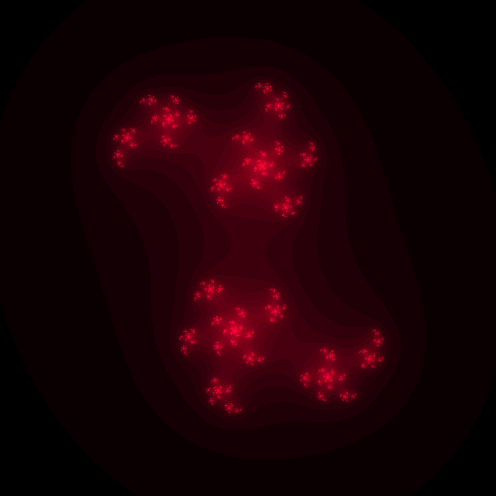
Here is a glow effect, meaning that the background is flipped to be the black portion.
You can also vary the zoom, although this needs some optimization to focus on interesting areas of the picture.

What Else?
The list I shared previously didn’t start like that. Every time I deemed myself to be “finished” I thought of something just a little cooler to do. And in fact, I still haven’t done everything that I wanted to do! But I have other things I want to work on, and need to stop somewhere. Here are some areas that could use improving:
Zoom
Currently, when you generate an animation with a varying zoom, it’s fairly arbitrary if we happen to zoom in to a point of the image that is interesting. For an improvement, when we generate an animation we might break the image into five quadrants (four corners and one center) and determine which has the most pixel entropy (the most differing pixels). This (maybe?) could be used to guess that there is something interesting going on here (as opposed to a uniform color that isn’t interesting to look at).
Infinite Zoom
These sets are known for those beautiful animations where you infinitely zoom, and I think this would be possible, given that we know the coordinate to zoom in on, and when to generate the next set animation. I haven’t thought about it much, but here it is if you want to take a crack at it, or even leave some notes or thoughts about it.
A Fun Project
I have one more little project up my sleeve that will use this library to make something interesting. I’m going to hold off from doing it today so I have something to look forward to this weekend. :)
I want to say thank you again to the author of the Color Julia Bot, I wouldn’t have delved into this if I didn’t see this cute little bot. It’s also an amazing example of how open source code can grow, and support really fun and awesome things! If you’d like to contribute, please open an issue!
Suggested Citation:
Sochat, Vanessa. "Juliart: Animations and Images for Julia Sets." @vsoch (blog), 27 Dec 2019, https://vsoch.github.io/2019/juliart/ (accessed 14 Jul 26).