wiki
Summer 2011
What is the connectivity between regions that have been known to have abnormal structure?
SPECIFIC AIMS
Are abnormal regions of structural connectivity connected functionally?
Mapping Meta-Analysis of VBM Studies Using Anatomic Likelihood Estimation (ALE) to Functional Networks
Attention Deficit Hyperactivity Disorder (ADHD) comprises a complex, heterogeneous set of disorders that affect 3-7% of school age children, leading to an estimated cost of $36 to $52 billion annually. Developing effective treatment and prevention requires a deeper understanding of the biological differences that characterize this disorder, e.g., differences in sex and structural connectivity in the human brain. While these measures are informative, a deeper understanding of the basis of variability among individuals diagnosed with ADHD calls for the integration of functional analysis. Our hypothesis is that abnormalities in structural connectivity will predict variation in functional networks, and that patterns of structural and functional dysfunction can ultimately be used to better characterize the behavioral and sex differences observed in ADHD.
This project aims to develop methods to relate deficits in structural connectivity to pathways of functional connectivity to summarize the relation of structural abnormalities to functional networks of the human brain. These methods will allow for a higher-level understanding of the functional basis of abnormalities in ADHD.
The specific aims of this project will include (1) building a machine-accessible database of extracted sMRI (structural MRI) data from ADHD patients, (2) summarizing deficits in structural connectivity, (3) using data-driven methods to infer functional connectivity networks , (4) finding overlap between patterns of structural abnormality and functional connectivity networks to functionally characterize ADHD deficits, and (5) to test this method by applying it to novel datasets and seeing if it reveals functional networks known to be affected in ADHD, and possibly networks not previously identified as being involved .
UPDATES
SEPTEMBER 13 UPDATE
As we are transitioning into the AIMify portion of this project and the summer quarter is over, all future updates will be posted - fall_2011.
SEPTEMBER 7 UPDATE
Things I have done:
Investigated Template Matching Script (SECTION 1 pyCorr ERRORS) Finished Testing pyVBM (SECTION 3 - pyVBM) Created magnitude neutral group network images and ran new dual regression (these maps are the ones to be “AIMified”) (SECTION 2- DUAL REGRESSION) Modified AIMTemplate to produce XML file for dual regression data see fall-2011
Working on:
I’d like to review the pyVBM results and make sure the empty images aren’t a result of me doing something wrong, then come to conclusions In the case they are empty, I’d like to run a GingerALE analysis with only younger age groups - could gray matter differences we see be a result of age?
Having Trouble With / Questions
What is a jacobian field? For niaim - it would be helpfull to have a better understanding of the big picture for XNAT and the XML files, and a concrete list of goals for the grant If we have no significant gray matter results, how do I summarize my project? Why do the absolute valued components lead to dual regression results that don’t include negative activations, still?
SECTION 1 - PYCORR ERRORS
It is clear that either something is weird with my python script, or the algorithm is responsible for the output. To test this, I decided to work with the 5th component as a template, since it is very easily identifiable, and I visually selected the “best match” component for each subject to have some sort of “gold standard.”
1) CHECKING FOR BACKWARDS RESULTS:
I ran pyCorr_Ks modified to print out ALL results (file IC5_match_result.ods and zthresh_stat.txt) and then located the “gold standard” within the entire distribution of the matches. It was very clear to me that the algorithm isn’t backwards (most of the “right” answers were in the top selected), however it was apparent that it simply WASN’T selecting for images that were better matches, for some reason. It is selecting empty images. However, it isn’t doing terribly… out of 10 subjects, the “right” component was in the top three for five of the subjects.
The question is, why are some empty images getting ranked higher than “potentially good” ones, and why doesn’t this happen with the V method? To investigate this, I opened up each of the “top choice” mostly images, and while a “normal” network has values between perhaps 0 and 15, all of mostly empty images have values closer to 100. So I think that the reason the algorithm gives them a higher score is because we have HUGE values in a very small number of voxels, so the activation per voxel not shared is HUGE! And then we subtract this huge number from a number close to zero (given there are essentially zero shared voxels), and then take the absolute value of that, leading to a larger number than, for example, a component with more overlap and voxels, but smaller values, which would mean working with overall smaller numbers (activation per voxel shared and not shared). The reason that taking the absolute value of the activation before adding it to the sum total leads the V method to not favor these empty images is because the activation per voxel is getting at the overall magnitude (both a positive 5 and negative 5 are considered equally interesting), which makes the average activation / voxel values relatively larger than if we were to add a positive 5, then subtract 5, and still divide by the same number of voxels. The V method also has high scores for the empty images with large values, however they don’t get pushed to the top because the other images average activation per voxel isn’t decreased by positive and negative activation values canceling each other out.
2) CHECKING FOR SCRIPT ISSUES:
My script could have a huge glaring error to be leading to the performance that we see for the K method, or perhaps the method and the utilization with nibabel has something going on, so I decided to run the NYU10 subjects through the same K method, but using the original script in MATLAB. I got the same results, to a T minus one subject (the 7th) that has nifti images with the first timepoint as blank. I’ve seen this happen once or twice with melodic, and it adjusts by writing the data to the second timepoint, which is shown and used in the report, so the user is never aware of it. When loading images into matlab or with nibabel, however, it is going to lead to an error! pyCorr accounts for this possibility, and uses the next time point if it finds an empty image, and the MATLAB script does not, which is why the result is different.
SECTION 2: DUAL REGRESSION
Took absolute value of all group components / networks (NYUALLABS.gica), and submit to run with another dual regression. This will do away with the issue of having activations / deactivations and needing to combine results, and it will be interesting to compare the three runs!
SECTION 3: PYVBM
Finished testing for NYU10, including the addition of the design.mat and design.con files for the design, and ran for NYUALL. The pipeline is as follows:
- Give script an output folder, contrast and design matrix, and an input file with subject IDs and paths to anatomical data
- Checks for files and paths
- Submit each single subject for preprocessing:
1) bet brain extraction .225 with skull cleanup
bet $OUTPUT/bet/${SUBID}_mprage $OUTPUT/bet/${SUBID}_mprage_bet -S -f 0.225
2) Mask the new BET image (but do not reduce FOV) on the basis of the standard space image that is transformed into the BET space
standard_space_roi $OUTPUT/bet/${SUBID}_mprage_bet $OUTPUT/bet/${SUBID}_cut -roiNONE -ssref ${FSLDIR}/data/standard/MNI152_T1_2mm_brain -altinput $OUTPUT/bet/${SUBID}_mprage_bet
3) Perform bet again on the standard registered cut image to get the final output
bet $OUTPUT/bet/${SUBID}_cut $OUTPUT/bet/${SUBID}_brain -f 0.225
4) Segmentation with FAST (segments a 3D image of the brain into different tissue types (Grey Matter, White Matter, CSF, etc.), whilst also correcting for spatial intensity variations (also known as bias field or RF inhomogeneities))
fast -R 0.3 -H 0.1 $OUTPUT/bet/${SUBID}_brain
R is spatial smoothing for mixel tyoe
H is spatial smoothing for segmentation
5) Register parameter estimation of GM to grey matter standard template (avg152T1_gray)
fsl_reg $OUTPUT/bet/${SUBID}_GM $GPRIORS $OUTPUT/bet/${SUBID}_GM_to_T -a
6) Wait until all single sub registrations complete! Then combine single subject templates into group gray matter template with affine registration
fslmerge -t template_4D_GM `ls *_GM_to_T.nii.gz`
fslmaths template_4D_GM -Tmean template_GM
fslswapdim template_GM -x y z template_GM_flipped
fslmaths template_GM -add template_GM_flipped -div 2 template_GM_init
7) Use fsl_reg with fnirt to register each single subject GM template to group GM template and standard space
for (( i = 0; i < ${#subids[*]}; i++ )); do
fsl_reg ${subids[i]}_GM template_GM_init ${subids[i]}_GM_to_T_init -a -fnirt "--config=GM_2_MNI152GM_2mm.cnf"
done
8) Take these single subject templates, now registered to standard space, and create a “second pass” group GM template
fslmerge -t template_4D_GM `ls *_GM_to_T_init.nii.gz`
fslmaths template_4D_GM -Tmean template_GM
fslswapdim template_GM -x y z template_GM_flipped
fslmaths template_GM -add template_GM_flipped -div 2 template_GM_final
9) Then when we have final template, submit each individual subject for second level processing. Register individual GM to group GM template final, jout is file for “Jacobian of field” for VBM
fsl_reg $OUTPUT/struc/${SUBID}_GM $OUTPUT/struc/template_GM_final $OUTPUT/struc/${SUBID}_GM_to_template_GM -fnirt "--config=GM_2_MNI152GM_2mm.cnf --jout=$OUTPUT/struc/${SUBID}_JAC_nl"
10) Take registered individual GM image and multiply by jacobian of field image (?)…
fslmaths $OUTPUT/struc/${SUBID}_GM_to_template_GM -mul $OUTPUT/struc/${SUBID}_JAC_nl $OUTPUT/struc/${SUBID}_GM_to_template_GM_mod -odt float
11) Wait for all single subject “round 2” to finish, and then merge both sets together…
fslmerge -t GM_merg `imglob ../struc/*_GM_to_template_GM.nii.gz`
fslmerge -t GM_mod_merg `imglob ../struc/*_GM_to_template_GM_mod.nii.gz`
12) Threshold the image at 0.01 and use GM_mask as a binary mask
fslmaths GM_merg -Tmean -thr 0.01 -bin GM_mask -odt char
13) Use fslmaths to integrate design matrix, contrast files, and then run randomise.
fslmaths $i -s $j ${i}_s${j}
randomise -i ${i}_s${j} -o ${i}_s${j} -m GM_mask -d $OUTPUT/tmp/design.mat -t $OUTPUT/tmp/design.con -V
for i in GM_mod_merg ; do
for j in 2 3 4 ; do
randomise -i ${i}_s${j} -o zstat_${i}_s${j} -m GM_mask -d $OUTPUT/tmp/design.mat -t $OUTPUT/tmp/design.con -n 5000 -T -V
done
done
14) Look at results (COMPLETELY EMPTY! :( ) For each of s2 s3 and s4… (resulting jacobian field images… what do s234 mean?) threshold the corrp images (corrected p value maps) at 0.95 to keep significant clusters and use it to mask corresponding tstats map:
fslmaths zstat_GM_mod_merg_s3_tfce_corrp_tstat1.nii.gz -thr 0.95 -bin mask_pcorrected3
fsl4.1-fslmaths zstat_GM_mod_merg_s3_tstat1.nii.gz -mas mask_pcorrected3.nii.gz fslvbms3_tstat1_corrected
fslview /usr/share/fsl/4.1/data/standard/MNI152_T1_2mm fslvbms3_tstat1_corrected.nii.gz -l Red-Yellow -b 2.3,4
Also did:
fsl4.1-randomise -i GM_mod_merg_s3.nii -m GM_mask -o fslvbm -d design.mat -t design.con -c 2.3 -n 5000 -V
Next steps:
calculate volume differences - but there are no significant results? I want to review the randomise command with K to make sure doing it right…
SEPTEMBER 2 UPDAT
THINGS I HAVE ACCOMPLISHED
- To come full circle with project - created pyVBM to derive structural differences from data see SECTION 1: VOXEL BASED MORPHOMETRY (pyVBM)
- Thinking about what constitutes a functional network SECTION 2: NEURODATA OBJECTS
- Installed XNAT on Rufus so we are ready to share a pipeline or dataset!
- Matlab runtime installed and tested on biox2 frontend2, and documented
- Working on reviewing ASD literature – SECTION 3- ASD PROJECT THINKING
- Organizing papers with Mendeley, awesome!
THINGS I NEED TO DO
- Complete testing of pyVBM –> run for NYUALL –> analyze results –> compare to functional data –> summarize / close up project
- When Dr Rubin has looked over basic XNAT, I’d like to try uploading data to understand how system works, and how we might use it
- In next few weeks - goal is to step back and broadly think about definition, extraction, and utilization of structural and functional biomarkers
QUESTIONS I HAVE
- Still want to choose best algorithm for matching template image (group network) to set of images (individual networks)
- When we are able to match - how do we use the individual’s network to better calculate correlations?
- Should we look for “closest” voxel coordinates, and extract from those regions? Should we try to get a measure of the strength of each side of the network? (size and strength right hemisphere vs left activation).
- It might be easiest to do simple correlations between activation in a network and a measure of structure - I haven’t finished the vbm so it’s not clear to me what the “results” data will look like.
SECTION 1- VOXEL BASED MORPHOMETRY (PyVBM)
This week I have mostly been working on an equivalent python method to derive my own structural measures, because meta analysis data isn’t combinable with functional networks. While I wanted to have finished results to look at for this update, job submission on the cluster has not been working, so I have not been able to produce this data. Hopefully this weekend things will be working smoothly and I will be able to run and analyze vbm results!
SECTION 2- NEURODATA OBJECT
I have been trying to mentally step away from the domain of a particular disease and think about the larger problem of analyzing and sharing large datasets. I attended David Chen’s final talk, where he talked about how he took large amounts of unstructured clinical data, and large amounts of structured genetic / hospital data, and was able to make connections between the two based on grouping by disease, age, gender, etc, and I think that the same might be done with neuroimaging data. My understanding is that you can take different domains (such as structural vs functional MRI), define biomarkers for each, extract a mean or median as a representative biomarker for a particular group (ADHD, ASD, male, female, etc), and then you might look at correlations between clusters of groups within the space of a different domains (a functional and structural marker, for example). I don’t see why we couldn’t do the same, and perhaps interesting inter-disorder patterns/trends might emerge.
The workflow to define biomarkers might go something like this:
Identify group biomarkers of structure (volumes (gm and wm)) and tract integrity (FA,MD,RD) Identifying group biomarkers of function (define and quantify networks, how “mirrored” activation and strength is, size, shape, etc) Decide on data structure to hold biomarker data, and extent to which relates to raw data (ideally it shouldn’t need to at all). My thinking is that any raw data might be run through a pipeline to generate the structures, and then the two can be completely separated. Given differences in scanners and aquisition protocol, it would be unlikely to combine raw data into one big analysis anyway. The purpose of this method would be to combine the modalities of structure, function, with demographic, behavioral, clinical, and possibly genetic data. If an interesting finding is observed, THEN would be the time to go back and do fine tuned analysis with raw data. Use the same process to extract biomarkers from the individual to compare to the group - the group vs individual objects should look the same.
This would require methods that can:
- 1) take different data types from raw format through generation of structures archive raw data somewhere (XNAT?) for download if someone wants to do analysis on a particular finding
- 2) make different structures queryable
- 3) efficiently do correlation analysis comparing biomarkers from two domains across any number of groups. Potential applications are as follows:
TO INDIVIDUAL DATA FOR DIAGNOSIS: upload single subject data, make conclusions about individual subject data BASED on findings derived from groups. TO GROUP DATA FOR RESEARCH: very quickly look at biomarker trends between domains, across many groups, for interesting patterns. The query might be as simple as looking at the relationship between average structural (volumetric) gray matter in the hippocampus and performance on a memory task for various groups, or more complicated, like the relationship between attention network activation and a measure of impulsivity, perhaps grouped by genotype. The idea is that you might observe a trend across many diseases, or across different genotypes or groups, and then you would be inclined to go back to the raw data and ask a very specific question.
The challenge and crux of this proposition is the definition of the biomarkers! It makes sense to start with functional and structural MRI, and to move from broadly defined to more specific groups. A good method should be usable across groups and data types, and should also be extendable to add other biomarkers.
FUNCTIONAL MRI
A method is needed to define and quantify networks, and then to allow for the calculation of a “difference” between an individual and a group derived network. For the individual, measuring a state of health or disease would be akin to comparing the individual score to all of the group scores. The group data object must be specific to the smallest unit we can query, the voxel level, to allow for complete freedom to define and compare individual and group networks. I haven’t thought this completely through yet, but I feel strongly that referencing an ROI is not specific enough. We need to have raw coordinate spaces with every single voxel, and in the case of functional networks, each voxel coordinate might be labeled via an ontology with a value that represents the probability of belonging to a specific network. If we know the voxelwise probability of networkness normality, then we can match an individual’s most likely attention network to a group “normal,” and then give points when an individual’s specific network overlaps the highly probable regions, and take away points when it overlaps a low probability region. The overall score at the end will tell us how much the individual network looks like the group network, and then we might rank and individual’s network across different group types and say “your attention network is most similar to that seen with ADHD, female, etc.” This method might be applied to the individual for diagnosis, or across groups. Each group object would include networks derived from ica, after filtering and further extraction of functional biomarkers.
Ideas for functional biomarkers of networks - a functional network object would contain:
- group ID derived from
- network name
- voxelwise probability scores of belonging
- Some measure of different hemisphere activation
- Some measure of where max activation is
- Some measure of strength of max activation
STRUCTURAL MRI
I can start thinking about when I finish VBM and am able to analyze results! In the future we should/will have molecular data about the brain, expression of genes in different parts, etc.
The goal is to have an object in each domain in each group that can be used to compare against the individual, and to look at correlations across domains for different groups / disease states, etc.
SECTION 3 - ASD (FALL) PROJECT THINKING
I am hopeful to be able to work on this general method of better creating, defining, and comparing functional and structural across domains. I would like to, for my next rotation, continue this work applied to ASDs. Dr. Reiss responded and said his RA would be in contact about an appointment, and my plan is to second a second inquiry if I haven’t heard by the evening of Friday September 2nd. My goal for this next rotation would be to do some integrated analysis with genetics, as I think that they are hugely important. To prepare I have started reading ASD literature, first with a review paper from Dr. Rubin, and from that I have downloaded 24 additional papers that I am working on reading. My take aways thus far is that it is astounding that there are differences on the molecular level, some which may not be completely driven by genes. This is telling me that we must make better methods for comparing these different modalities.
When we have structural and functional markers, and are looking for genetic data I have found this as a resource –> http://research.agre.org/
AUGUST 26 UPDATE
THINGS I HAVE ACCOMPLISHED
- Overview of method for template matching - SECTION 1- METHOD OVERVIEW
- Created python script to do matching for 2 methods (pyCorr 1 and pyCorr 2), and pyCorrPrint to print HTML report
- Visually summarized - results - SECTION 2 - VISUALIZATION OF RESULTS
THINGS I WANT TO TRY
- Creating a gold standard for the components, and a confusion matrix to show accuracy - SECTION 3 - GOLD STANDARD PROPOSAL
- Using matched networks somehow to better calculate correlations on the individual subject level for networks
QUESTIONS I HAVE
Which method for matching components should we use / how might we decide? What is the best way to create a “gold standard”
SECTION 1 - OVERVIEW OF METHOD
As a reminder, the rationale behind needing this method is to better match group networks to individual networks, and to then calculate correlations based on the individual’s network, instead of jumping back to raw, noisy data. To do this in an efficient manner, we need a method to calculate spatial correlation between two images.
- First I wanted to look at the source code for fslcc (which requires images of same size) to see if I could recreate functionality in matlab or python. I learned immediately that it is calculating the correlation based on values in timeseries, and isn’t a tool for spatial location, so it’s not what I want.
- I decided that we needed a simple method to read in an image, figure out the locations that were important, transform those locations to MNI space, and then see if the same locations had activation in an image we were trying to match. At this point I was very lucky because K sent me doTemplateMatching.m, which is the standard for doing this sort of spatial correlation. Thank you K!
Summary of method:
- Read in images
- Find spots that meet some user specified threshold
- Look up spots in each image you are trying to match
- For shared activation, add one to a shared activation voxel count, and add the value to a shared activation total
- Set all spots equal to zero and then search for any remaining activation (activation in image but outside template)
- Create an equivalent unshared activation voxel count and value total
- Calculate an activation difference score
- Rank scores in descending order and choose top three
Analysis of Method
Find indices for the template image where it meets some criteria. In this case, where it is equal to an intensity of 200. These indices will be for voxels that are in the template.
indexes = find( Y == roi_intensity );
For each index that we find in the template, we then check the same spot in each component image. When we find a voxel with an activation that isn’t zero, we add one to our voxel count of voxels in the roi, and add the activation value of the component to activation_in_roi. These two values represent overlap.
for i=1:numel(indexes)
if Y1(indexes(i)) ~= 0
activation_in_roi = activation_in_roi + Y1(indexes(i));
voxel_in_roi = voxel_in_roi+1;
Here are are setting all of the indices that represent areas of the template that we’ve already counted in the component to zero so that we can look for activation outside the template. I would assume that activation outside the template would be an indication of not matching as well!
Y1(indexes) = 0;
for i=1:numel(Y)
if any datapoint is not equal to zero after we have accounted for the template areas, this is activation outside the template, and we add 1 to our voxel_out_roi count, and add the activation itself to activation_out_roi. It’s not clear to me why we are enumerating through the number of points in Y (the template) as opposed to the component that we are looking at, but it seems that since they are assumed to be the same size, it doesn’t matter.
if Y1(i) ~= 0
activation_out_roi = activation_out_roi+Y1(i);
voxel_out_roi = voxel_out_roi+1;
We now have two sets of measures. “in_roi” represents matching activation, positive or negative, and “out_roi” represents “extra” activation that is in the component image, but not the template. Again, I would assume this means not matching. We now calculate the difference between the two…
activation_difference(jj) = (activation_in_roi/voxel_in_roi) - (activation_out_roi/voxel_out_roi);
Activation per voxel shared - Activation per voxel not shared (and I’m not sure how/if we are accounting for areas in the template that don’t have activation at all in the component image, another indication of not matching. If the activation per voxel shared is larger than the activation per voxel not shared, then the value is positive, and that’s good, because the overlapping voxels, regardless of the number, are relatively higher in activation. However if the activation per voxels not shared is larger, then the activation difference is negative, and that’s not as good, because it means that the average activation per voxel in the areas that don’t fall within the mask are relatively higher… the activation in the component doesn’t match the template!
If we maintained the positive and negative signs, that would make sense. But here is where I got confused! We are taking this activation difference, and taking the absolute value, and THEN sorting. So an activation difference of -10, meaning the average activation per voxel in areas that don’t fall in the mask is larger than activation that does fall in the mask, is getting ranked equally with a score of positive 10, the activation per voxels for areas within the template. This is what I didn’t/don’t understand!
% Compute the top 3 similarity score components
[comp_sort_descend idx] = sort(abs(activation_difference),'descend');
If I were trying to match an activation image to a template, I would give points for activation in areas that are within the template, and take points away for activation in areas outside the template, OR areas without activation within the template.
Example of Why Method Might Need Change
(shared activation / voxel shared) - (unshared activation / voxel not shared)
So the larger the value this is, the better, because we want there to be more shared activation per voxel. I think that the assumption here is that we are working with components that are largely positive or largely negative, and I’m more worried that the abs() score calculation when done with a component that is a mixture won’t be a good representation of how well it fits the template…
Scenario 1: All positive or all negative
Given that a component is largely deactivation (negative Z values) or activation (positive Z values) - the calculation makes perfect sense:
A) A "matching image that is primarily positive activation in and outside template would have":
(Large positive value) - (Small positive value) = Still positive value
10 - 2 = 8
B) A “matching image that is primarily negative activation in and outside template would have”: (Large negative value) - (small negative value) = Still positive value -10 - (-2) = -10 + 2 = -8 </code> Then when you take the absolute value, they are equivalent, and can be ranked equivalently.., this is good!
Scenario 2: A mix of positive and negative
I think that it’s more likely that components have a mix of negative and positive activation - and if we just want to find the best fit, at least for the simiarity calculation, we shouldn’t care about the direction. So in this scenario, we have a mix of negative and positive Z values:
C) A "matching image that has primarily positive activation w/in template, negative outside:
(Large positive value) - (Small negative value) = A bigger value than if the activation outside was + 10 - (-2) = 10 + 2 = 12 (this image would be ranked as a better match than example A, even though they are the same, one just has deactivation outside instead of activation!
D) A “matching image that is primarily negative activation w/in template, positive outside”: (Large negative value) - (small positive value) = higher negative value -10 - (2) = -12 so when we take the absolute value it is ranked as a better match than A or B </code>
Proposal
So I’d like to propose the following change: that we look at the magnitude of the Z value as being most important for indicating a strong fit, and when we add the activation value to the total, we take the absolute value at that point. So we would do:
% if voxel has activation and is within template:
voxel_in_roi = voxel_in_roi + 1
activation_in_roi = activation_in_roi + abs( new_activation_value ) '''if voxel has activation and is outside template'''
voxel_out_roi = voxel_out_roi + 1
activation_out_roi = activation_out_roi + abs( new_activation_value )
…then when we calculate activation difference, we won’t need to take abs() again, and can rank the scores in descending order, and the highest value means there is the highest absolute activation per shared voxel…. a match!
activation_difference = (shared activation / voxel shared) - (unshared activation / voxel not shared)
SECTION 2 - VISUAL COMPARISON
I created a python script to create results reports, which can be seen - here
SECTION 3 - CREATION OF GOLD STANDARD
I knew I would be getting output of top three matching images from individual subjects to group networks, so I needed a gold standard to compare my results to. I created a simple excel sheet, and listed the group network components for the NYU10, and then used these functional ROIs (based on my own judgment) as templates for the different networks. I need to do this for every group network (30 of them) for each of the NYU10, so I am not far along in doing this. I thought that it would be best to discuss before I jumped into anything!
AUGUST 16 UPDATE
THINGS I HAVE ACCOMPLISHED
- processing / dual regression for NYUALL group (N = 178)
- visual analysis of spatial correlation, and anatomical labeling NYUALL maps
- method to extract timeseries of max voxels from dual regression results
- started using glmnet to attempt to predict ADHD diagnosis from correlations (MACHINE LEARNING SECTION 1)
- project summary and figures (K MEETING SECTION 2)
- method to ica_corr.m calculate all correlations between significant voxels in components (CORRELATION MODELS SECTION 3)
THINGS I WANT TO TRY
- overlay positive and negative dual regression activation results in same space and visually look for overlap with structural meta results.
-
I recently found a python module ([ PyNifti](http://niftilib.sourceforge.net/pynifti) that can manipulate nifti images! (it utilizes the C libraries I think). It’s predecessor seems to be [ NiBabel](http://nipy.sourceforge.net/nibabel/), although for now I have downloaded the original. I really want to give it a try, because this could mean easy integration of imaging data with numpy, scipy, and another library I found called matplotlib, which allows for matlab-like plotting via python. Tackling a problem like getting images in the same space, or calculating spatial correlation, might be better done through a library like this one! - I also want to read this paper to get an example application of glmnet and accessing its performance.
QUESTIONS I HAVE
- I still don’t have a grasp of a statistical / mathematical method for calculating spatial correlation between a dual regression results and structural map, to “quantify” the functional / structural overlap. my attempts at registration to use fslcc from previous weeks were unsuccessful, so my next idea is to see what I can do with PyNifti.
- I was hoping to hear back from K about “good” components so I can filter out bad ones, and re-run models. I could also use my own judgment, but I also wanted to get his expertise on the networks themselves, which we talked about.
SECTION 1: MACHINE LEARNING PROPOSAL
I have never done machine learning before, but I think that it would be interesting to see if we can use extracted BOLD values to predict ADHD status. It seems that most algorithms take in an “input vector” - or a 1 X N matrix of predictor variables, and commonly the “outcome” (1 for ADHD, or 0 for control, for example) is appended to the end.
With this format in mind, I have created a melodic_ts script that goes through the results of dual regression analysis (from a group melodic) done with ica+, and extracts the top ten local max coordinates for each specified dual regression result. These are voxel coordinates. It then goes back to single subject ica runs and extracts the timeseries for each of the local maximum voxels, and prints them all to a text file in the following format:
EXTRACTED TIMESERIES EXAMPLE - 4 subjects, two clusters, N Timepts.
C1_TP1 C!_TP2 C1_TP3 … C2_TPN C2_TP1 C2_TP2 C2_TP3 … C2_TPN C1_TP1 C!_TP2 C1_TP3 … C2_TPN C2_TP1 C2_TP2 C2_TP3 … C2_TPN C1_TP1 C!_TP2 C1_TP3 … C2_TPN C2_TP1 C2_TP2 C2_TP3 … C2_TPN C1_TP1 C!_TP2 C1_TP3 … C2_TPN C2_TP1 C2_TP2 C2_TP3 … C2_TPN </code> The output also includes a text file with the voxel coordinates, for later reference.
CHOICE OF ALGORITHM
I spoke with Francisco about this idea, because he seems to know a lot about machine learning, and he suggested that I use the GLMnet algorithm, called “lasso” - which is good for datasets with a large number of input variables because it tries to maximize assigning “0” values to the weights of variables, which might tell us which cluster values are “richest” in conveying information about ADHD diagnosis. I found that I could use the algorithm through R and Matlab, chose matlab, and first wrote a script to read in an output text file from my ica+ pipeline and run one model, and then to - batch process it, and then finally to take the structure of models created by the batch and run a prediction for each one.
I first created models using the NYU10 as training data, but thought that the small sample size wasn’t ideal. I decided to use the NYUALL dataset (178 individuals), and split it into 150 for training, and 28 for testing. To start, my outcome variable was ADHD or CONTROL, and the default of glmnet is to do a gaussian model, which I believe to be linear regression, which I think about as having a bunch of data points, and wanting to draw a straight line through them to “best fit” the data, meaning that we want to minimize the distance between each point and the line. My understanding is that the algorithm is trying to find the coefficient to go with each predictor input to define this line, and you can think of this like a weight. At the same time, it is trying to assign as many weights of zero to the input components to find a solution with the minimal number of predictors.
I didn’t know about the technique of folding the data, so at this point I used 150 NYUALL subjects to train with the extracted timeseries for each subject for each component as input. The result was a model for each component, and then I could test each model on the 28 subject training set. I also wasn’t sure how to calculate the accuracy of the model beyond comparing the predictions with the actual, so I chose to do that to display my first set of results (detailed below).
RESULT OF GAUSSIAN GLMNET MODELS
This chart shows the raw prediction scores for each subject across the 28 component models..
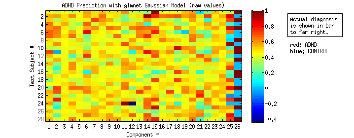
I then rounded each raw score to either 0 or 1, based on which it was closer to to get a “binary prediction snapshot.”
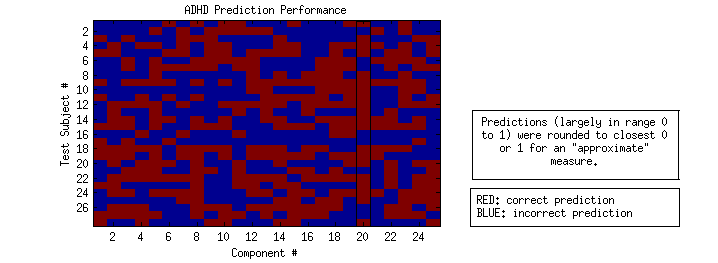
Based on this rough method, the top performing model was created from component 20, with a correct prediction rate of ~70% (black box).
I then went back to the dual regression components, and cool! Component number 20 is clearly an attention network and the dual regression analysis that shows significant differences within this network has max voxels located in Broadman’s area 10 and 13, which is in the medial and superior frontal gyrus of the frontal lobe. This is awesome!
SECTION 2: MEETING WITH K
At this point I decided to stick with working with the larger NYU dataset, and I produced the FSL coordinates, MNI coordinates, Talarch coordinates, and all of the dual regression result and network anatomical regions for reference. I then met with K and we discussed the following:
- Ordered List Itemwhere / how to calculate accuracy. He sent me a snippet of code to modify glmnet to include accuracy, and it looks like we do this (and choose a lamda) by taking in a list to try, keeping track of the squared error for each one, and choosing the one with the highest validation accuracy.
- a statistical method for assessing spatial correlation: I think he said that he would have a script to send me, but I never heard, so perhaps I misunderstood him.
- filtering “bad” components: We did about 9 quickly in person but K stopped me and said that he would send me an email. This is important for setting up the models with only “good” components. I haven’t heard back, but as soon as I do I want to re-run models without “bad” components to see if performance improves.
- combining all components into one model: We agreed I would try creating models for both individual and combined components. Since I didn’t hear back from him, I ran the compiled models with all components with the rationale that the bad “noise” ones would get eliminated by the algorithm (given weights of zero). We also talked about choosing max voxel coordinates based on having a unique anatomical label, so I would convert coordinates to talaraich space to assign labels, and choose unique ones within each component. I again haven’t done this yet because I don’t know which components are “good” - but I am ready to better summarize results.
- I had noticed that our dual regression results didn’t capture significant deactivations (the blue areas of the component maps that represent the contrast (ADHD > Control). If you look at the NYUALL report, it is very salient that these blue areas never overlap with significant dual regression results, and this is because the contrast is set to have a weight of 1. I don’t think that we completely understand how to think about this contrast, but my gut was to think about the areas as significantly “deactivated” for ADHD as compared to controls. I think that these are just as important, so I ran it by K, and I created another dual regression run to capture these points (a contrast with weight -1), and do the same with extracting timeseries and calculating correlations for use with machine learning models.
- very important - K informed me that my first attempt at machine learning was wrong, and he is right. By using the extracted timeseries as the input data, I am saying that a random point in time for subject N is equivalent to the same point in time as subject N+1, which is not right. Instead, we decided to use correlations between significant points in each network for the input vector, for both each component individually, and all of them combined. This is detailed in SECTION 3
- he also asked me to write up a project summary with a few figures for Sunday or at the latest, Monday, so I spent the weekend doing that. This was really fun to create the Figures, and a good exercise in summarizing a lot of work into a few pages. It gave me insight to how important it is to keep a record of the details of your work, and your sources!
SECTION 3: CORRELATION MODELS FOR “ACTIVATIONS”
My goal was to create correlation matrices for each of the sets of local max voxel coordinates for each of the 25 components for each subject.
- Use this scripts to extract complete timeseries for each component’s group of local max values
- I wrote a matlab script that will take these timeseries, and calculate the correlation between each local max and output them to file, either with or without the P-value (see script for details). I then used the correlation matrices as the input vector for new models with glmnet, and - ran the models using the modified script from K, which takes an entire dataset and breaks it into a user specified number of folds (k), a number of lambdas to try, calculates prediction accuracy for each, and then creates the actual model with the highest cross validation accuracy (best_cva). This is the measure that I used to access the accuracy of the models, and my results are as follows, after running for both activations and deactivations for individual components:
COM#      Activations (ADHD > Control)   Deactivations (Control > ADHD)
1         0.5235                         0.5118
2         0.5765                         0.5824
3         0.5588                         0.5353
4         0.5647                         0.5294
5         0.5882                         0.5647
6         0.5294                         0.5294
7         0.5118                         0.5412
8         0.5529                         0.5176
9         0.5353                         0.5412
10        0.5353                         0.5471
11        0.5529                         0.5353
12        0.5353                         0.6059
13        0.5353                         0.5235
14        0.5294                         0.5353
15        0.5353                         0.5353
16        0.6                            0.5529
17        0.5412                         0.5529
18        0.5353                         0.5176
19        0.5294                         0.5294
20        0.5235                         0.5706
21        0.5647                         0.5647
22        0.5706                         0.5882
23        0.5353                         0.5471
24        0.5529                         0.5353
25        0.5294                         0.5294
note that components between activations and deactivations do not line up!
The general accuracy was between 55 and 60% - eyeing the numbers it looks like the deactivation correlations led to a slight improvement, but not great. These results are only slightly better than chance. I then combined all correlations into one model (for activations, deactivations, and both), and the result was slightly improved.
Control (1) and ADHD (2)
All deactivations       0.5588
All activations         0.5529
BOTH                    0.6294
I then decided to try using ADHD subtype for my outcome list instead of a binary status, and the models actually dropped into the high 40’s for accuracy, so I steered clear away of that for now. I don’t think that I know enough about the statistics behind the models (yet!) to know what algorithm is best to use, and how to customize that algorithm. I’m very eager for classes to give me some guidance in this regard, and grateful that I was able to have my first machine learning experience with this summer rotation project.
EXTRA LEARNING
I also downloaded and tested WEKA, which seems to be a popular plug and play machine learning toolbox, although it does not have the GLMnet lasso algorithm. I used the extracted timeseries from component 1 and formatted my input data into an .arff file that the software expects, and was surprised to see that some classifiers (SVG based) can have a successful prediction rate of 100%, and others can drop down to 30%-50%. It was also interesting to see that, for this sample component, algorithms that attempted to identify the most meaningful input data consistently used values from a particular voxel, as opposed to a combination of voxels. I was hoping for a combination of voxels, to represent a network.
AUGUST 8 UPDATE
The goal is to make meaningful connections between the meta analysis (representing significant regions of structural differences between ADHD and control) and the dual regression results (representing significant differences in functional networks). I wanted to use a tool called fslcc, which takes two input images and reports a spatial correlation, and the images of course should be in the same space, orientation, and size. Our two sets of data do not fit these requirements, so for the first part of my weekend work I attempted again to re-orient and register the images.
REGISTRATION AND ORIENTATION to prep for spatial correlation
The images can be summarized as follows (name, description, orientation, dimensions, voxel size)
- MNI152_T1_2mm_brain.nii.gz –> MNI standard template, LAS 91 X 109 X 91 2mm vox
- Colin27_T1_seg_MNI.nii –> MNI standard template, RAS, 151 X 188 X 154 1mm vox
- gm_wm_input_p05.nii –> Gingerale thresholded output, RAS 77 X 96 X 79 2mm vox
- dr_stage3* –> dual regression result, LAS 45 X 54 X 45 4mm vox
I’m surprised that the Colin MNI template is being suggested for use with the GingerALE output, saying that the dimensions are different. This might work for visualization with MRIcron or work in SPM, but certainly not with FSL.
Opening them with MRIcron, they all line up nicely, which makes sense given that they are all in MNI space. The problem (in terms of using fslcc) is one of orientation (right to left needs to be switched) and then the image needs to be trimmed. I took the following steps to fix the orientation.
- 1) Check the origins. Since they line up, it must be because they have a common origin (as in, where the files originated from). I decided to use the display tool in SPM to get the origins of each.
MNI152_T1_2mm_brain.nii.gz ---- 46 64 37
Colin27_T1_seg_MNI.nii     ---- 76 112 69   (ACPC)
gm_wm_input_p05.nii        ---- 39 57 36
dr_stage3*                 ---- 46 64 37
Since the dr_stage3 has the same origin and orientation as the MNI standard template (I’d be worried if it didn’t!), it makes sense to work with those two images. First I will flip the gm_wm_input_p05 from left to right.
fslswapdim gm_wm_input_p05.nii -x y z gm_LAS
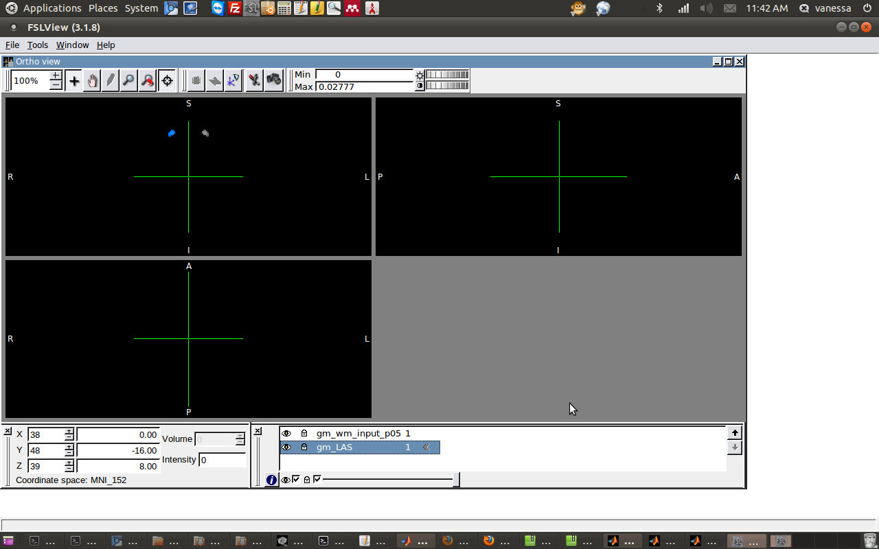
2) Force neurological (changing header info).
This first command will return a “NEUROLOGICAL” report when you do:
fslorient -getorient gm_LAS.nii.gz
Now here I will change the header info by switching the sign in the sform and copying it to the qform.
fslorient -copysform2qform gmLAS.nii.gz fslorient -setsform -2 0 0 76 0 2 0 -112 0 0 2 -70 0 0 0 1 gm_LAS.nii.gz fslorient -copysform2qform gmLAS.nii.gz
The values correspond to the sform and qform matrices, which I believe tell us how to read the raw image data. Since an image itself is just a flat list of numbers, we can only assign coordinates and put it into a 3D space if we know how to read the data, which I think is the purpose of the header, period. For example, if I switch the sign in the raw data for x to switch from left to right, if I don’t change the header info, it won’t reflect the change. I am just starting to learn about this, and it seems to me you have to be super careful when doing anything with orientation. You have to change the data AND the header! The sform matrix usually represents how to get the image into standard space (I think)!
Now the image correctly displays and reads to be in LAS, neurological convention. Now I will give another try to registering the gm_LAS image to the standard template! Linear registration should be OK, so I will use FLIRT.
3) Reattempt Registration
3a) First register the dual regression result to the MNI template
flirt -in /../Desktop/gmALE/test/reg/dr_stage3_ic0021_tfce_corrp_tstat1.nii.gz -ref /../Desktop/gmALE/test/reg/MNI152_T1_2mm_brain.nii.gz -out /../Desktop/gmALE/test/reg/dr_stage3_standard.nii.gz -omat /../Desktop/gmALE/test/reg/dr_stage3_standard.mat -bins 256 -cost corratio -searchrx -90 90 -searchry -90 90 -searchrz -90 90 -dof 12 -interp trilinear
3b) Then register the gm_LAS image to the MNI template
flirt -in /../Desktop/gmALE/test/reg/gm_LAS.nii.gz -ref /../Desktop/gmALE/test/reg/MNI152_T1_2mm_brain.nii.gz -out /../Desktop/gmALE/test/reg/gm_LAS_standard.nii.gz -omat /../Desktop/gmALE/test/reg/gm_LAS_standard.mat -bins 256 -cost corratio -searchrx -90 90 -searchry -90 90 -searchrz -90 90 -dof 12 -interp trilinear
3c) Now attempt to overlay the two output… although the two images now can be displayed together on the standard space, it’s obvious that they were incorrectly warped. This was the output, which is just wrong!
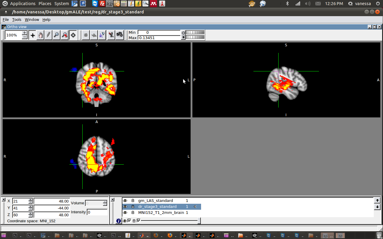
I decided to try linear registration, but with only 9 DOF, which is called “Traditional” instead of “Affine” transformation. I think this means that the algorithm can translate,stretch, but not change the voxel size. This also came out, in a word, wrong.
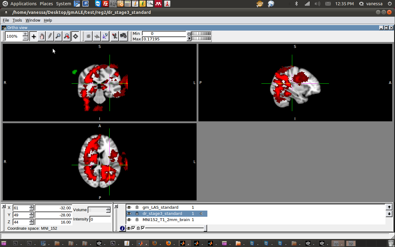
I gave one more effort and tried to do FNIRT, which is nonlinear registration, and had another failed attempt - the output images are completely empty!
SPATIAL CORRELATION - VISUALLY DETERMINED
I think that I’m doing something horribly wrong for this to not work, but I don’t want to get stuck here. My goal is to have an understanding of how the gingerALE output relates to the dual regression output. I have first tried to relate the two by putting them into the same space, and I’m having a lot of trouble. This is unfortunately the current state of neuroimaging - there are always different orientations / sizes / spaces, and the goal is to be able to make connections between these different images. It is very easy when data is collected from the same scanner (and common), and not so much if that isn’t the case! The purpose of MNI space, it seems, is to be able to make these connections, regardless of image size, resolution, and voxel size. If two images are both in MNI space, we can be confident that the coordinates are talking about the same spot in the brain. So for my next attempted solution, I want to forget about getting the images exactly the same, and find a way to relate them in a human friendly way, based on anatomical labels.
Anatomical Labeling for any Nifti Image My goal now is to provide anatomical labels for my dual regression results and meta analysis image, and then look for overlap, and if the labels “make sense” given the current research about functional deficits in ADHD. There isn’t a tool that automatically provides labels for any nifti file - there are only around the bush ways. SPM has a toolbox called aal that allows this functionality, but only with an SPM.mat. FSL lets you load an image and click around to see the probability of belonging to a certain image based on an atlas, but that isn’t very batchable. I think it would be a good project to create a tool that can take in any nifti image and automatically label it, but for the purpose of my project, I am going to label by extracting the local maxima, and then converting MNI coordinates to talarach space using GingerALE, and then looking up the labels with the the Talarach daemon.
Extraction of Local Maxima from Dual Regression Results
- 1) melodic_ts: I was making this script to extract local maxima from dual regression results to play around with machine learning, and I think I can have it save these local maxima to file for use with looking up regions with the talarach demon.
-
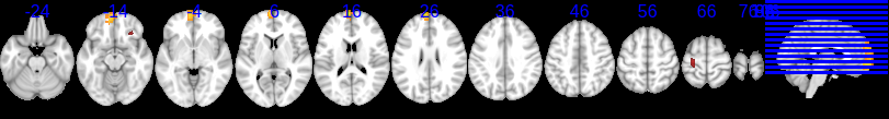
2) I have extracted the local maxima from each of the 30 dual regression results from the new bandpass NYU10 run, used the converter provided in GingerALE to convert from MNI to talarach, and prepared my findings in a web report. I still wanted to overlay the structural deficit image on the dual regression results, so I cheated and used MRIcron, which does not care about image size, and does a very good job of making sure images (even multiple overlays) are displayed in the correct orientation. I opened each respective “standard space” image for the dual regression results and the structural meta analysis (the MNI 152 2mm brain template, and the Colin MNI brain template, respectively), and since these lined up perfectly in MRIcron, I decided it would be safe to overlay my structural and functional results. I have included these images in the web report, along with the original functional networks, for comparison.
- NYU10 is the report that contains my visual conclusions about overlap between the structural result and the functional network.
I must note that I finished this on Sunday August 8th, however had to go back and redo everything when I noticed on Monday that the regions reported were all in the right side of the brain. I then retraced my steps, and noticed that all of my MNI coordinates were positive (this isn’t right because we definitely have significant results on the LEFT side of the brain, represented by a negative x value), and then it hit me that the tool I used to extract the values (cluster, via fsl) is in fact giving VOXEL coordinate reports. I read about this, and in order to get them in standard space (MNI) I need to multiply each set by the sform matrix. I extracted the sform matrix from one of the dual regression output images (this is the same for all dual regression results) and wrote a quick matlab script to do the conversion. I then went back to the talarach demon and regenerated my list of anatomical regions, and was happy to see more accurate results! I will be more careful about this next time, because I lost about half a days work time!
NEXT STEPS and Questions!
While I think that a few components potentially overlap, most do not. For our next steps, here are some ideas:
- I definitely want to know your thoughts on the structural and functional overlap! Also, I never heard from K about the bandpass results…
- Now that I’m getting a better understanding of images / headers, I’d like to propose writing a matlab script that can calculate spatial correlation between nifti images of different sizes. I also wanted to ask K how he calculates spatial correlation… I wanted to make one of those beautifully colored matrices, and even after reading many papers that include them, I didn’t understand how.
- I really want to try the machine learning algorithms to predict ADHD status from these results!
- How can we filter out “bad” components, in a logical / data driven way?
- Can we use our dual regression results in another way? I read an article about how different genes are expressed differently in the brain - could we see if there is any significant correlation with our ADHD/Control differences?
- Do we keep working with NYU10?
AUGUST 5 UPDATE
Overview of Implementation of Bandpass Filtering
At our last meeting we discussed a new work strategy of taking things one step at a time, and we agreed that the next step to take was to work on bandpass filtering. K sent me the matlab script on Tuesday that utilizes the Matlab Signal Processing Toolbox (thank you! :D), and so the past two days the focus has been to:
- create a wrapper that takes in a nifti as input, reads the image, bandpass filters, and writes the new image.
- build all the necessary .m scripts into a package, and compile
- test / run the bandpass filtering on the cluster via the Matlab Runtime Compiler
Step 1
Step 1 was not too difficult. I decided to use the Nifti / Analzye toolbox to read in the image, extract the data and header information, convert from single to double values (required by the bandpass script), perform bandpassing, and then extract information from the old header for the filtered data to be as accurate as possible. Lastly, I saved the new image. I modified the melodic_ss.sh script to perform the filtering, and was sure to leave the old method there (commented out), in the case it was needed. Since the input and output for this new bandpass method must be .nii and we are working with .nii.gz with the rest of the pipeline, in melodic_ss.sh I also used fslchfiletype before and after. The entire new “bandpass section” is now as follows:
Bandpass filter the data using matlab executable, bandpass
First convert the .nii.gz to .nii
fslchfiletype NIFTI prefiltered_func_data_intnorm.nii.gz
Launch matlab script ( <input .nii> <name for output .nii (no extension)> <TR>
$SCRIPTDIR/run_Bandpass.sh $MATLABRUNTIME prefiltered_func_data_intnorm.nii prefiltered_func_data_tempfilt $TR $LFILT $UFILT
The output will be .nii, which we need to change back to .nii.gz
fslchfiletype NIFTI_GZ prefiltered_func_data_tempfilt.nii
Use fslmaths to copy the file with a new name (filtered_func_data)
fslmaths prefiltered_func_data_tempfilt filtered_func_data </code>
Step 2
I struggled with step 2. It wasn’t clear that the standalone executable that matlab produces is dependent on the platform, so I was trying and reading everything to produce a linux executable from Windows, and I could not figure it out. I created the C and C++ libraries and was trying to compile them on my own, but having never done compilation before, was having a hard time. It wasn’t until K mentioned that “a deploytool on unix shall produce a shell script” that I finally installed matlab on my Mac (producing a .sh and .app) and then finally on linux (Ubuntu) producing a linux executable and .sh. As a review of the output of this process and the command above:
- run_Bandpass.sh: Is a shell script that takes the path to the MCR ($MATLABRUNTIME), followed by variables needed by the main .m script (input nifti, then output name, then the TR and filter lower threshold and filter upper threshold). It sets up the MCR environment, and submits the executable with your input arguments
- Bandpass: is the executable itself. Compiled on Mac produces a .app, on Windows produces a .exe, and on linux produces a linux executable (no extension)
- $MATLABRUNTIME: is the Matlab Runtime Executable, which can be produced by any matlab installation if you run the executable “MCIInstaller.*” under matlabdirectory/toolbox/compiler/deploy/ It produces a runtime compiler that matches the version / OS the original scripts were built and compiled with. This is where I ran into my next set of problems.
Step 3
The version and OS that the script is compiled from has to be exactly the same as the MRC, so I was unable to get my compilation to work with three MCR versions that K had previously used. I was also unable to install the same version of matlab on my linux machine, because I am running 32 bit, and the versions were 64 bit. I tried to modify the libraries in a copy of the existing MCRs to work with my version, but it became very apparent that the errors would be rampant, and it would make most sense to use an MCR from the same installation the scripts were compiled from. I decided to create my own MCR from my installation, and this worked great until I exceeded my quota when trying to install it on the cluster. The saving grace at the end was K compiling the scripts on his machine, and using his old compiler with the matching version on Wednesday night.
Informatics Takeaways
Utilizing matlab code in this manner would be incredibly difficult if not impossible for most users, and so adding bandpass filtering in this format is not ideal for anything other than our personal usage.
Question for K: Being able to compile matlab scripts for running on the cluster is something that I’d like to be able to do, as it will be very useful during my graduate career. If you have some free time, could we talk about how you were able to install the MCR given the quota limits?
Processing NYU10 with Correct Bandpassing
I have re-done the NYU10 (single subject ICA, QA checking, group ICA, and dual regression) with the ica+ pipeline. I am so grateful for having this pipeline, otherwise this process would have taken days instead of an hour or so!
Now that we have the correctly filtered data, I would like to propose that we continue with our strategy and talk about the next steps for comparing the dual regression output with the structural output. Here are some things that I was trying on my own (from our meeting last week, before K sent me the bandpass scripts Tuesday) that might be in the right direction. I will include all things, even if they didn’t turn out to be successful.
NEXT STEPS AND THINGS EXPLORED
1) Dual Regression Results:
I didn’t feel that I had a good idea of how the dual regression results compared with the original functional networks, so I wanted a way to visualize the thresholded, p corrected dual regression output (the areas of each functional network that are significantly different between control and ADHD) versus the original networks themselves. I added to the dual regression script to automatically produce a web page with images of the DR output overlayed on the network, sliced in various orientations, and although it accomplishes the goal, I’m not happy with the results. it is much more meaningful and useful to open up a pair of images in FSL. If I have extra time I would want to improve this visualization, because output like this would greatly contribute to my understanding. I stopped working on this after a day and a half when I determined it wasn’t essential to my project.
2) Calculating Spatial Correlation:
It makes sense to me that we would want to calculate the correlation between the dual regression output and the structural image produced from the meta analysis. The only way that I currently know how to try doing this (likely not a good one :P) is by using fslcc, which takes two identically oriented and sized images, and calculates the spatial correlation. I spent a few days figuring out how to change the group ALE output (in Neurological orientation, and different dimensions) to the FSL standard (Radiological). This requires using fslswapdim to first change the data itself, and then fslorient to change the header to match.
fslswapdim rest_input -X Y Z rest_LAS    # swap the x dimension to change left and right
fslorient -forceradiological rest_LAS
fslorient -copysform2qform rest_LAS
fslorient -setsform -2 0 0 90 0 2 0 -216 0 0 2 -72 0 0 0 1 rest_LAS
I then used the same process with flirt to get the structural meta analysis image into the standard space, and a sample dual regression output as well - except instead of registering raw data to the standard with the high res anatomical as intermediate, I tried registering the meta to the dual regression with the standard as intermediate. It produced an empty image, so it didn’t work. I am going to keep trying things to see if I can get this to work - perhaps using the MNI template that the Ginger ALE team provides on the site (Colin27_T1_seg_MNI.nii). My thinking is that, since both are in MNI space (but just different image sizes) - it probablty makes most sense to use method that figures out a correlation based on voxel coordinates, regardless of image size. I feel empowered to try things using either FSL or something with matlab. Can we talk about the best way to go about doing this spatial correlation?
3) Predicting ADHD Diagnosis with Extracted BOLD values:
I read a network analysis paper that looked at the impact of health status on friendships, and while I wasn’t so interested in that particular application, it occurred to me that I could apply this sort of method to the ADHD dataset, using (for the training dataset) the ADHD diagnosis as the “outcome” and extracted BOLD values as the prediction vector. I have the basic understanding of the input data, and thought that I might learn about machine learning by playing around with it, so I wrote a script for the ica+ package that does the following: For each dual regression result (component) specified by the user:
- Extracts the local maximum voxel coordinates, including their Z value and which cluster they belong to, and prints to a summary file, if needed later.
- Goes to single subject data, extracts the full timeseries at each voxel
- Produces an output text file, one per component, with each row corresponding to one subject, containing a list of (176 timepoints) X (N timeseries significant voxels)
For example, the output below would be for three subjects, for one component / dual regression result. 1,2,3 would correspond to a significant voxel, and TP1,TP2,TP3, timepoints 1 to 3.
(Subject 1)   1_TP1, 1_TP2, 1,TP3...2_TP1, 2_TP2, 2_TP3...n_TP1, n_TP2, n_TP3
(Subject 2)   1_TP1, 1_TP2, 1,TP3...2_TP1, 2_TP2, 2_TP3...n_TP1, n_TP2, n_TP3
(Subject 3)   1_TP1, 1_TP2, 1,TP3...2_TP1, 2_TP2, 2_TP3...n_TP1, n_TP2, n_TP3
I would then figure out how to use this data as training data with the ADHD diagnosis being the outcome, and come up with an algorithm that can be given values extracted from these groups of coordinates, and come up with an ADHD diagnosis. I ran this idea by K, and he said that he’s already done it, but I’d still like to, even if it’s just a personal project :O) I spoke with Francisco today and he pointed me toward Weka as a good starting point for a “machine learning GUI” - and then recommended trying out GLMnet with he lasso algorithm, which tries to weight as many of the inputs in the prediction vector with 0 as possible to get a better result. I am just downloading the software as we speak so I don’t have anything to report beyond that! And I understand that this is not applicable to my main project, so I will always prioritize it second.
Summary Functional networks have now been correctly bandpass filtered, and I’d like to move swiftly to the next steps. Since this is less big picture and more “which tool should I use,” I think that email exchange should suffice! I’d like to utilize the weekend to work, especially given the past week feeling unproductive due to the challenges above, so if at all possible could we discuss this today or tomorrow?
JULY 28 UPDATE
This past week I have been working on optimizing the method so that we can reproduce it for the entire NYU dataset. I’ve made a python submission script that works with several lower level scripts to perform individual ICA, group ICA, Quality Checking, and Dual regression. Full documentation of the scripts can be found here, and document the process for the NYU10 dataset here (the output which we are discussing this week). I want to note that I am NOT publicly posting the scripts or any documentation that references data paths, as I am sensitive about the potential proprietary nature of this work!
DOCUMENTATION OF RUNNING FOR NYU10
Created input file with 10 subjects csv file with subject ID, full anatomical data path, full functional data path. This is the only preparatory step that needs to be done before running the scripts.
1) SINGLE SUBJECT ICA
This performs the single subject processing
python2.4 ica+.py –o /../Analysis/Group/NYU10_auto –ica=rawinput.txt
Checking for FSL installation…
Output directory already exists.
Reading input data file…
Checking for all anatomical raw data…
Checking for all functional raw data…
Checking for LAS orientation of anatomical data…
Checking for equal timepoints between functional input…
The number of timepoints for all runs is 176
Checking for LAS orientation of functional data…
Creating output directory /../Analysis/Group/NYU10_auto/ica…
Job <579400> is submitted to default queue
2) OUTPUT OF SINGLE SUBJECT ICA
The result of running the above is an “ica” and “list” folder in my specified output directory. In the “ica” folder I have a subfolder for each subject (sub1.ica, sub2.ica, etc) and in the “list” folder I have a copy of my raw data input file, as well as a (date)_ica.txt file, which has a list of the ica directories, which is what I will use as the input file for the next step, running quality analysis.
3) QUALITY ANALYSIS
Quality Analysis can be run using the python submission script (recommended) or stand alone. It basically finds the file prefiltered_func_data_mcf.par, which contains six columns, the xyz rotational and translational motion across time (each row is a timepoint), and flags any subject that exceeds a user specified threshold. We decided to use 2mm of translational motion, or 2 degrees of rotation.
This command uses the output file of the first step as input to run Quality Analysis, and the output will be named “qaall”
python2.4 ica+.py –o /../Analysis/Group/NYU10_auto –qa=/../Analysis/Group/NYU10_auto/list/2011-07-26_14_25_ica.txt –name=qaall Checking for FSL installation… Output directory already exists. Checking for output directory… Output directory /../Analysis/Group/NYU10_auto already created. Creating output directory /../Analysis/Group/NYU10_auto/qa… Creating output directory /../Analysis/Group/NYU10_auto/qa/log… Found all mc/prefiltered_func_data_mcf.par files… Job <583332> is submitted to default queue
. </code> From running QA, I see that no subjects are flagged for having a gross amount of motion, for either rotation or translation in xyz. I should note that in my test runs I manually changed test data so it wouldn't pass QA, and the script flagged these subjects.
4) GROUP ICA
Since my subject list hasn’t changed, I could again use the list/_ica.txt file as input for group ICA, or I could use the list/_qa.txt file, which contains subjects that pass QA.
python2.4 ica+.py –o /../Analysis/Group/NYU10_auto –gica=/../Analysis/Group/NYU10_auto/list/qaall_qa.txt –name=NYU10ALL Checking for FSL installation… Output directory already exists. Reading ICA directory input… Creating output directory /../Analysis/Group/NYU10_auto/gica… Creating output directory /../Analysis/Group/NYU10_auto/gica/NYU10ALL.gica… Creating output directory /../Analysis/Group/NYU10_auto/gica/NYU10ALL.gica/log… Job <583448> is submitted to default queue
. Done submitting GICA job. Follow output at /../Analysis/Group/NYU10_auto/gica/ </code>
6) DUAL REGRESSION
The next step will be dual regression, however we need to discuss the GICA output first. This Wednesday I modified the submission script to perform dual regression, and created a design matrix to specify one condition: Diagnosis, and I set ADHD = 1, and CONTROL = 0. Here is he command and output for the NYU10 dataset:
python2.4 ica+.py -o /../Analysis/Group/NYU10_auto –dr=NYU10ALL.gica –name=NYU10ALL –con=/../Analysis/Group/VTEST/DESIGN/NYU10.con –mat=/../Analysis/Group/VTEST/DESIGN/NYU10.mat –iter=500 </code>
UPDATE - JULY 15, 2011
GRAY MATTER SIGNIFICANT DIFFERENCES
- gm_wm_volume.xlsx: contains voxel coordinates for grey, white, some FA from papers
- have prepared image with GingerALE - no region lookup
Functional Network Derivation - Step 1: ICA Method in MELODIC
- downloaded all ~800 ADHD datasets and put on scratch
- first did single subject ICA, K pointed me in direction of dual regression, which I read is done after a Multi session temporal concatenation. My understanding of this method is that it takes subject 2D datasets (space over time) and stacks them on top of each other, and THEN does an ICA analysis. So the components that come out represent timecourses that are common amongst subjects, instead of a single ICA, which is only timecourses relevant to one subject. Then, a design matrix can be applied at the next step, dual regression (should we do everyone or separate control from ADHD, and derive common components for each group?)
Functional Network Derivation - Step 2: Preprocessing
Since we will be combining functional data right off the bat, I first investigated registration that needs to happen BEFORE ICA. MELODIC will perform brain extraction and motion correction on functional data, and you can specify registration to a highres for a single run ICA, but when doing the multi session temporal concatenation, you can’t specify the unique highres for each subject. So registration of the functional data to the highres and standard space would need to happen before MELODIC is run.
REGISTRATION
- FLIRT registration: is FSLs tool for linear registration. I first did BET on the highres and then FLIRT to align the functional resting data to the highres (for all subjects), but then read papers and saw they ALSO aligned to standard space, and didn’t use FLIRT.
- FNIRT registration: is FSLs tool for non-linear registration, which I read can do a better job for registering large groups of subjects into same space. So I did a brain extraction on all hires anatomicals, then used FNIRT to register the functional to the highres, the highres to standard, and then combine the parameters to get a matrix to align the functional to standard (with highres as a sort of intermediate)
#------------------------------------------------------------BET Brain Extraction
#———————————————————— echo “Performing BET brain extraction on “ $ANATFILE bet $ANATPATH/$ANATFILE.nii.gz $ANATPATH/mprage_bet.nii.gz -S -f .225 #————————————————————-
FLIRT LINEAR REGISTRATION
#————————————————————- echo “Registering “ $FUNCDATA “ to mprage_bet” flirt -ref $ANATPATH/mprage_bet.nii.gz -in $FUNCDATA.nii.gz -dof 7 -omat $FUNCDATA”_func2struct.mat”; flirt -ref ${FSLDIR}/data/standard/MNI152_T1_2mm_brain -in $ANATPATH/mprage_bet.nii.gz -omat $ANATPATH/affine_trans.mat; fnirt –in=$ANATPATH/$ANATFILE.nii.gz –aff=$ANATPATH/affine_trans.mat –cout=$ANATPATH/nonlinear_trans –config=T1_2_MNI152_2mm applywarp –ref=${FSLDIR}/data/standard/MNI152_T1_2mm –in=$FUNCDATA.nii.gz –warp=$ANATPATH/nonlinear_trans –premat=$FUNCDATA”_func2struct.mat” –out=$FUNCDATA”_warped_func”;
Old script to use FLIRT to register the brain extracted anatomical to the resting data
#flirt -in $FUNCDATA.nii.gz -ref $ANATPATH/mprage_bet.nii.gz -out $FUNCDATA”_coreghires.nii.gz” -omat $FUNCDATA”_cogreghires.mat” -bins 256 -cost corratio -searchrx -90 90 -searchry -90 90 -searchrz -90 90 -dof 12 -interp trilinear </code> Comparison of FNIRT to non-registered data. I ran a MELODIC multi-session temporal concatenation analysis for just the Brown dataset (26 subjects, no speficiation of ADHD/Control) with only aligning functional data to standard space. I then used FLIRT to create the resting data warped to the highres and standard, and ran another MELODIC multi-session temporal analysis with these as input. The registered images are better / correct, hands down, and I feel silly for trying a run without registration!
Functional Network Derivation - Step 3: Dual Regression
I read about Dual Regression and found this paper and this paper that utilize the method. The steps were to pre-process, perform the multi-session temporal-ICA, and then setup a general linear model with GLM or a similar method - as long as you have a design matrix and contrast files.
Dual Regression Test Run:
Since I wanted to do a test run with the Brown dataset, I made a mock design file and contrasts, and ran the dual regression script. I didn’t add any contrasts other than a group mean, since the dual_regression script simply does a randomise function, which I believe is a one sample T-Test. I’m not sure what the design matrix should look like - we should talk about this! I did 500 permutations, which I think corresponds to a p value of .002. The command is as follows (for local machine):
./dual_regression.sh /Users/vanessa/Desktop/mnt/scratch/Project/ADHD/Analysis/Group/BRN_BET.gica/groupmelodic.ica/melodic_IC 1 /Users/vanessa/Desktop/mnt/scratch/Project/ADHD/Scripts/DESIGN/BRN_BET/BRN_BET.mat /Users/vanessa/Desktop/mnt/scratch/Project/ADHD/Scripts/DESIGN/BRN_BET/BRN_BET.con 500 /Users/vanessa/Desktop/mnt/scratch/Project/ADHD/Analysis/Group/BRN_DUAL_REG `cat /Users/vanessa/Desktop/mnt/scratch/Project/ADHD/Analysis/Group/BRN_BET.gica/.filelist`
Output of dual regression is as follows:
- dr_stage1_subject(#).txt: one text file per subject, each has columns of timecourses, one coln = the timecourse for one component
- dr_stage2_subject(#).nii.gz: spatial maps outputs of stage 2 of the dual regression. Each subject has one image like this, and it is a 4D image - with one 3D image (one timepoint) representing one component. So the number of timepoints = number of components. This 4D image is the “parameter estimate” image.
- dr_stage2_subject(#)Z.nii.gz: same as above, but the Z stat version
- dr_stage2_ic(#).nii.gz: a 4D image of all subject parameter estimates for one component. So it’s the same as the parameter estimate images, but reorganized by group ICA component, and one 3D image corresponds to one subject. This image is used as input for the next stage, “cross subject modelling for each ICA component”
- dr_stage_3ic(3)_tstat(#CON).nii.gz: the output of the final stage! running FSL’s randomise “Doing cross subject statistics for each group ICA component. There would be one image per contrast per component, but since we only have one contrast (group mean), we only have one image / component.
We are interested in the tstat images, and finding the higheset correlation between each image (representing a single component across subjects) and our gray matter “template” image). The tstat images are dependent on the design matrix and the number of permutations run, so I’d like to talk about these things.
Functional Network Derivation - Step 4: Overlapping Networks
We are interested in the “tstat” need strategy to find how significant structural findings overlay on these group networks. I read that a criticism of ICA analysis is that many of the networks are noise, or related to some other biological process. Proving that the structural deficits map onto one of more of the functional networks is evidence that they are in fact neuronal related!
This first command takes the gray matter structural findings image (from GingerALE) and transforms it into the same space as one of the melodic outputs (same dimensions, voxel size)
flirt -ref thresh_zstat1.nii.gz -in gm_input_p05.nii -out gm_p05_thresh_reg -nosearch -interp trilinear
Now use fslcc to find the spatial correlation between two images (for each of our output from dual regression and the gray matter image)
for i in {1..9}; do echo $i `fslcc gm_p05_thresh_reg.nii DUALREG_stage3/dr_stage3_ic000$i"_tfce_corrp_tstat1.nii.gz" 0`; done
for i in {10..90}; do echo $i `fslcc gm_p05_thresh_reg.nii DUALREG_stage3/dr_stage3_ic00$i"_tfce_corrp_tstat1.nii.gz" 0`; done
Identify Functionally Deviant Areas in each Network Across Subjects, and Find Spatial Correlation to META image of Structural deficits
- Running dual regression is applying a GLM to the ICA maps. The GLM (as is setup now) just creates one big group, and a group mean contrast.
- Randomise command takes the GLM and basically does a one sample T test)
- tstat output image (one for each component) is cross subject statistics for each ICA component, and we want to find spatial correlation between these images and the gm volume image. These images represent areas in each component (network) that are deviant from the mean, in a group of ADHD/control this might be the “aberrant” network activity. We want to see the spatial correlation between these functionally aberrant areas and the gray matter deficits.
We have identified top functional networks that map on to structural meta analysis findings… now what? crickets*
Current State of Data: all ~800 datasets have brain extracted anatomicals, and rest warped to highres and standard
Next Steps - Solidifying Group Design and Included Data
- First I’d like to suggest reviewing all steps of the Brown dataset, and talk about what the images mean, and it would be helpful for K to share his expertise! At some point I also want to review the design matrices that I used / thresholds. etc.
- We will need to both solidify the data, the design, and the method!
Defining a Definitive Dataset (out of 800)
- We need to select a definitive dataset. This decision is based on the following:
- I don’t think we can combine datasets with different number of timepoints / TR - we could only cut datasets
- do we want to set an equal number of controls / ADHD?
- does any subtype of ADHD = ADHD diagnosis (1) vs control (0)? Do we even need to specify this anywhere, since it’s a data driven approach?
- After step 2 I’d like to review the setup of the MELODIC and the design matrix / contrasts!
Reading: The Elements of Statistical Learning
UPDATE - JUNE 17, 2011
(extension of June 8th update)
- completed reading meta analysis papers (7)
- found all papers from one meta, and reading through them - completed ~13
- got frustrated with excel and keeping things organized - going to result in un-usable product!
- decided to make matlab data structure instead (more object oriented)
- wanted to query data - matlab not good for that, decided on MySQL
- created MySQL database & matlab script to convert different structures to import statements
- have moved information from excel –> matlab structure –> mysql database for query
- Next: Learn queries to ask simple questions (based on decided project)
- Map question types to fields that should be searched
- For measures / regions - integrate ontologies
- Continue to read papers and add results
- if decide is useful - build simple front end with PHP and let others test.
- End goal –> to use database to drive / support hypotheses, improve if is effective tool
NEUROSCIENCE SIDE UPDATE takeaway / interesting ideas from reading (ADHD)
Age / Developmental Stage
- in-utero variables also linked to developing ADHD (alcohol, mother age, fT)
- child brain defined by small world networks, global ones reinforced normal development
- reduced volume fronto-striatal regions in ADHD can improve into adulthood, & w/ meds
- steep increases FA right up until adulthood, slows down (DB13)
- Hormones (fT, differences M/F) must have influence on brain development
Gender
- studies are biased towards children and male, M/F should be separated
- females show earlier maturation white matter compared to males (RD) (DB13)
Volume Differences
- both cortical thinning and reduced volume of fronto-striatal regions
- cerebellar volume is significantly smaller - reduction continues over time
White Matter Connectivity
- FA: overall significant and similar increase in FA with age in both ADHD and control groups, but specifically localized regions of difference in the ADHD group (DB12)
- They didn’t find significant differences in FA when using TBSS (mean/center of fiber tracts) but Ashtari did (who didn’t use TBSS) - could the loss be happening at the edges? Maybe instead we WANT to look at the edges?
- Overall Our question of focus is “What is the connectivity between regions that have been known to have abnormal structure” and I think a subquestion to that worth investigating is “Why do these regions have abnormal structure?” My current project is putting together a database with information about abnormal structure in ADHD and then use my database to further identify structural patterns and then look at connectivity between those regions. It seems salient to me that both white and gray matter volume differences are global, and given the significant influence of both gender and period of development, I think the most interesting things to look at might have to do with hormonal influences on the structure of the brain. Could hormones or the function of the choroid plexus in maintaining proper homeostasis, lead to differences in neurogenesis, and slow structural changes over time influence function? The following project proposals are all related to these questions exploring the relationship between structural and functional connectivity, and hopefully getting at the “why” behind the whole thing using methods that integrate bioinformatics.
Things to look at based on individual ideas / observations
- CSF / Choroid Plexus via Cerebellum
- Hormonal Influences on Structure
CSF / Choroid Plexus via Cerebellum:
why does no one think about it, given that the choroid plexus and ependyma cells constitute the blood brain barrier, responsible for filtering out bad stuff, and maintaining homeostasis? Could it be the case that if you have something slightly off about this system… so maybe the choroid plexus influences hormone levels, or doesn’t filter out toxins as well, and that harms the ependyma cells over time, and then that has direct consequences for the white matter that is closer to ventricles. 1) Given that there is significant volume reductions in the cerebellum and (choroid plexus is down there at 4th ventricle) - could it be the case that proximity to csf / CP is positively correlated with a structural difference?
- look at significant findings of structural abnormality and compare to CP/CSF proximity (database)
- see if there is relationship between gray and white matter deficits and CP / CSF (our dataset)2) OR perhaps we could even have a case of areas of the brain closer to CP and ventricles (cerebellum) get worn down over time and that propogates to other regions. if we see consistent volume reductions in the vermis, which is the epicenter of the choroid plexus, does that say that something is happening close to there?
- since cerebellum is so innervated by CP, could segment into tiny pieces and compare volumes and connectivity to other associated networks (our dataset)
- look at others significant findings related to cerebellum and see if matches our findings (database)3) If proximity to CSF is important, then might it be the case that the perimeter of a tract is more “vulnerable” than the center? TBSS (which uses mean / center FA skeleton for a group) shows no significant difference between ADHD/control, while differences emerge when you look at the whole tract.
- within groups - compare FA values in the center vs edges of a tract, and then see if the differences are significantly different between groups (gender and ADHD scale) (our dataset).
- see if using FSL –> TBSS (with a mean skeleton) influences the result (database)WHY
- If we find significant differences between M/F for any of the above - could track development of the CP, and look for differences in NT levels or genetics that could account for gender differencesHormonal (Gender) Influence on Structure:
- create list of hormones / proteins influential for neurogenesis expressed in the brain
- figure out where they are strongly expressed
- look for significant structural differences in those areas between ADHD/control, M/F, using both an informatics approach (asking database) and with our own dataset
- Could we map expression to structure, and then hypothesize how that alters function?
Aromatase CYP19A1: catalyses conversion of T to estradiol, effects exerted through E receptors.RORA - retinoic acid-related orphan receptor-alpha - converts T into estradiol. Expression of RORA and aromatase found to be highly correlated.Testosterone - Higher fT exposure leads to “increasing rightward asymmetry in the isthmus (projects to posterior parietal and superior temporal cortices) , which are integral for language and visuospatial ability and are known to be sexually dimorphic in lateralization, structure, and function” – “An animal model of ADHD suggests that early androgen exposure affects catecholamine innervation of the frontal cortex and cognitive function” (Baron-Cohen, 2011) Transthyretin (TTR) carrier protein for thyroxine (T4) - main hormone synthesized by the thyroid gland - biologically active principle of T4 is T3, and activity of this enzyme is regulated in the CNS so T3 levels are stable. Thyroid hormones essential for normal growth of the CNS! The liver and the CP are major sources of TTR - choroidal epithelium starts synthesis of TTR at an early stage of brain development. “TTR also can be produced in the hippocampus, most likely by neurons, in response to various experimental manipulations” CASK Peripheral plasma membrane protein - “multidomain scaffolding protein with a role in synaptic transmembrane protein anchoring and ion channel trafficking” on short arm X chromosomeACSL4 Long-chain-fatty-acid - activation of long-chain fatty acids for both synthesis of cellular lipids, and degradation via beta-oxidation. Involved with dendridic spine architecture? Proteolipid (PLP) and basic (MBP) that make up Myelin - need to research these!Steroid sulfatase (protein catalyzes the conversion of sulfated steroid precursors to estrogens during pregnancy)Monoamine oxidase-B ( plays an important role in the metabolism of neuroactive and vasoactive amines in the central nervous system and peripheral tissues and degrades dopamine) SRY (initiates M sex determination) - expressed in medial rostral hypothalamus, frontal / temporal regions. “SRY can increase transcription of tyrosine hydroxylase (rate-limiting enzyme in dopamine biosynthesis) by binding at a promoter site … knockdown of SRY expression in the substantia nigra of the rat decreases tyrosine hydroxylase expression… could implicate SRY in the male bias for disorders involving disregulated catecholamines such as ADHD… SRY may also regulate the monoamine oxidase A (MAO-A) gene” (Baron-Cohen 2011).