Neuroscientists need to understand their results in the context of previous literature. If you spit out a brain statistical map from your software of choice, you might have any of the following questions:
- How consistent is the result?
- How specific are the brain regions(s) to the task?
- Does co-activation occur between… regions? studies?
Toward this goal, we have methods for “meta-analysis,” and for neuroimaging studies there are two types: coordinate (“peak”) based meta-analysis (CBMA) and image-based meta analysis (IBMA). The current neuroimaging result landscape is dominated by peaks, but now with growing databases of whole-brain maps we have entire mountains, and it’s this new interesting problem of needing to perform inference over these mountains.
Recently I wanted to learn about meta-analysis approaches for coordinate data. I’ll be brief because I have much more I want to read, but I wanted to give a shout out to a figure (from a different paper) that really helped to solidify my understanding of the CBMA methods. I won’t re-iterate the methods themselves (please see the paper linked above), but they are broadly kernel density analysis (KDA), activation likelihood estimation (ALE) by way of GingerALE, and multi-level kernel density analysis (MKDA) that addresses some limitations of the first two (and don’t forget about NeuroSynth that mines these coordinates from papers and gives you tools to do meta-analysis!). This figure below comes from a paper by Salimi-Khorshidi et. al. that wanted to compare these common CBMA approaches to IBMA.
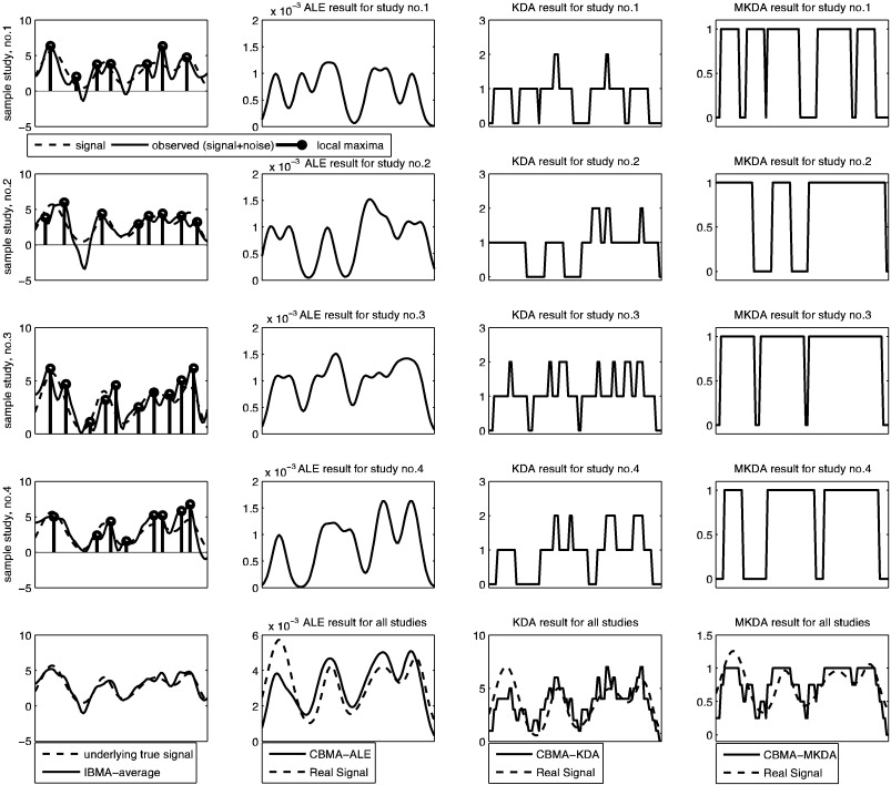
An illustration of ALE vs KDA vs MKDA (CBMA approaches) vs IBMA
I really appreciated this image for showing the differences between these CBMA (coordinate based meta analysis) approaches and then an image based meta analysis. I think that we are looking at method score/output on the x-axis, and voxels on the Y.
Each of first three rows contains a simulated dataset. The “true” signal is the dashed line, and then the bold lines in the first column of each row are that signal with added noise (imagine that there is some “true” signal underlying a cognitive experience that all three studies are measuring, and then we add different noise to that). The dots would be the “extracted peak coordinates” reported in some papers (and this is the data that would go into some CBMA). So each of the first three rows is a simulated study, and within those rows, the first column shows the “raw” data and “peaks,” and the last three columns are each of the CBMA approaches. In the last row, we see how the methods perform for meta-analysis across ALL the studies – however the very bottom left figure shows that the IBMA (averaging over the images) produces a signal that is closest to the original data, and this looks a lot better than the CBMA approaches (columns, 2,3,4). In summary:
- column 1: is the raw data, with the big black dots showing the local maxima that are reported, dotted line is “true” simulated signal, black thick line is that signal with added noise.
- column 2: shows the results of ALE: the result is more of a curve because the “ALE statistic” reflects a probability value that at least one peak is within r mm of each voxel, so the highest values of course correspond to actual peaks.
- column 3: kernel density analysis (KDA) gives us a value at each voxel that represent the number of peaks within r mm of that voxel. If we divide by voxel resolution we can turn that into a “density”
- column 4: is MULTI kernel density analysis, which is the same as KDA, but the procedure is done for each study. The resulting “contrast indicator maps” are either 1 (yes, there is a peak within r mm) or 0 (nope).
Please read the papers to get a much better explanation. I just wanted to document this figure, because I really liked it. The whole thing!
Suggested Citation:
Sochat, Vanessa. "Visual explanation of coordinate-based meta-analysis approaches." @vsoch (blog), 08 Jan 2015, https://vsoch.github.io/2015/visual-explanation-of-coordinate-based-meta-analysis-approaches/ (accessed 14 Jul 26).